Ship-Ship Collision Calculations

This chapter describes OMRAT’s calculations for ship-ship collision risk. Five encounter types are modelled – head-on, overtaking, crossing, merging and bend – based on the equations in Pedersen (1995) and Friis-Hansen (2008).

Overview

Ship-ship collisions occur when two vessels occupy the same space at the same time. The IWRAP methodology models this by calculating the geometric number of collision candidates – the expected number of close encounters per year assuming no evasive action – and then multiplying by a causation factor to get the actual accident frequency.

The general formula is:

\[F_{\text{collision}} = N_G \times P_C\]

Where:

• \(N_G\) = geometric collision candidates per year

• \(P_C\) = causation probability (IALA default values)

Pipeline orchestrator: compute/ship_collision_model.py:1224 – run_ship_collision_model()

Head-On Collisions

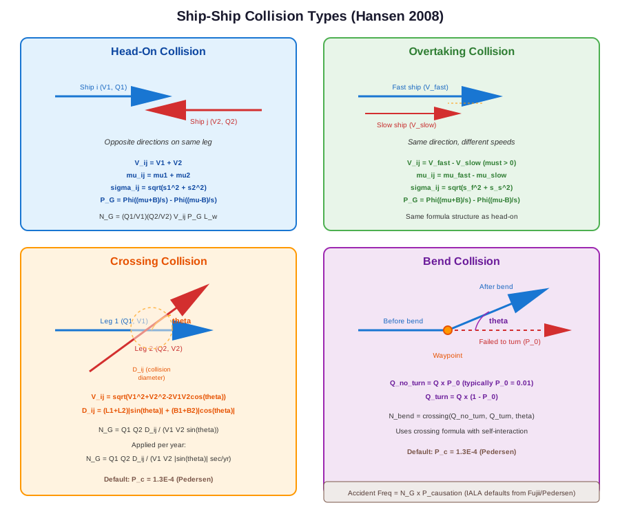
Head-on collisions occur between vessels travelling in opposite directions on the same leg. This is the classical encounter type for narrow shipping lanes.

Geometry

Two streams of traffic travel in opposite directions. The collision probability depends on the lateral overlap of their position distributions.

Equations (Hansen Eq. 4.2–4.4)

The geometric number of collision candidates is:

\[N_G = \frac{Q_1}{V_1} \times \frac{Q_2}{V_2} \times V_{ij} \times P_G \times L_w \times \frac{1}{\text{sec/year}}\]

Where:

• \(Q_1, Q_2\) = traffic volume in each direction (ships/year)

• \(V_1, V_2\) = vessel speeds (m/s)

• \(V_{ij} = V_1 + V_2\) = relative closing speed (m/s)

• \(L_w\) = leg segment length (m)

• \(P_G\) = geometric collision probability

The term \(Q/V\) converts from traffic frequency (ships/year) to traffic density (ships/m), accounting for the time ships spend on the leg.

The geometric collision probability is:

\[P_G = \Phi\!\left(\frac{\mu_{ij} + B_{ij}}{\sigma_{ij}}\right) - \Phi\!\left(\frac{\mu_{ij} - B_{ij}}{\sigma_{ij}}\right)\]

Where:

• \(\mu_{ij} = \mu_1 + \mu_2\) – combined mean lateral distance (head-on: positions add because ships face opposite directions)

• \(\sigma_{ij} = \sqrt{\sigma_1^2 + \sigma_2^2}\) – combined standard deviation

• \(B_{ij} = (B_1 + B_2) / 2\) – average vessel breadth (collision width)

• \(\Phi\) = standard normal CDF

compute/basic_equations.py:329 – get_head_on_collision_candidates()

Head-on collision candidate calculation (compute/basic_equations.py)

def get_head_on_collision_candidates(
    Q1: float,           # Traffic in direction 1 (ships/year)
    Q2: float,           # Traffic in direction 2 (ships/year)
    V1: float,           # Speed direction 1 (m/s)
    V2: float,           # Speed direction 2 (m/s)
    mu1: float,          # Mean lateral position dir 1 (m)
    mu2: float,          # Mean lateral position dir 2 (m)
    sigma1: float,       # Std dev lateral position dir 1 (m)
    sigma2: float,       # Std dev lateral position dir 2 (m)
    B1: float,           # Beam of vessel type 1 (m)
    B2: float,           # Beam of vessel type 2 (m)
    L_w: float           # Leg segment length (m)
) -> float:
    """
    Calculate geometric number of head-on collision candidates.

    Uses Hansen Eq. 4.2-4.4:
    N_G = Q1 × Q2 × V_ij × P_G × L_w

    Where:
    - V_ij = V1 + V2 (relative closing speed for head-on)
    - P_G = Φ((μ_ij + B_ij)/σ_ij) - Φ((μ_ij - B_ij)/σ_ij)
    - μ_ij = μ1 + μ2 (mean lateral distance between vessels)
    - σ_ij = √(σ1² + σ2²) (combined standard deviation)
    - B_ij = (B1 + B2)/2 (average vessel breadth)

    Parameters
    ----------
    Q1 : float
        Traffic in direction 1 (ships/year)
    Q2 : float
        Traffic in direction 2 (ships/year)
    V1 : float
        Speed direction 1 (m/s)
    V2 : float
        Speed direction 2 (m/s)
    mu1 : float
        Mean lateral position dir 1 (m)
    mu2 : float
        Mean lateral position dir 2 (m)
    sigma1 : float
        Std dev lateral position dir 1 (m)
    sigma2 : float
        Std dev lateral position dir 2 (m)
    B1 : float
        Beam of vessel type 1 (m)
    B2 : float
        Beam of vessel type 2 (m)
    L_w : float
        Leg segment length (m)

    Returns
    -------
    float
        Geometric number of head-on collision candidates per year
    """
    # Relative closing speed for head-on collision
    V_ij = V1 + V2

    # Mean lateral separation between vessels (head-on: opposite directions).
    # Hansen Eq. 4.4: mu_ij = mu_i^(1) + mu_j^(2), both positive from own
    # sailing perspective.  OMRAT stores dir-2 means negated to a fixed
    # reference frame, so we subtract to recover the Hansen convention.
    mu_ij = mu1 - mu2

    # Combined standard deviation
    sigma_ij = sqrt(sigma1**2 + sigma2**2)

    # Average vessel breadth (collision width)
    B_ij = (B1 + B2) / 2

    # Geometric collision probability using cumulative normal distribution
    # P_G = Φ((μ_ij + B_ij)/σ_ij) - Φ((μ_ij - B_ij)/σ_ij)
    if sigma_ij > 0:
        P_G = norm.cdf((mu_ij + B_ij) / sigma_ij) - norm.cdf((mu_ij - B_ij) / sigma_ij)
    else:
        # If no variance, check if collision is certain (within beam)
        P_G = 1.0 if np_abs(mu_ij) <= B_ij else 0.0

    # Number of geometric collision candidates
    # Hansen Eq. 4.2-4.4:
    # N_G = (Q1/V1) × (Q2/V2) × V_ij × P_G × L_w
    # Where Q/V converts frequency (ships/year) to density (ships/meter)
    # This gives the correct dimension: collision candidates per year

    # Avoid division by zero
    if V1 <= 0 or V2 <= 0:
        return 0.0

    # Convert to ships per meter (density)
    # Q is ships/year, V is m/s, so Q/V gives ships/year / (m/s) = ships * s / (year * m)
    # We need to convert: ships/year / (m/year) to get ships/m
    # V_year = V * seconds_per_year
    seconds_per_year = 365.25 * 24 * 3600
    density1 = Q1 / (V1 * seconds_per_year)  # ships per meter
    density2 = Q2 / (V2 * seconds_per_year)  # ships per meter

    # N_G = density1 × density2 × V_ij × P_G × L_w × seconds_per_year
    # This gives collision candidates per year
    N_G = density1 * density2 * V_ij * P_G * L_w * seconds_per_year

    return N_G

Default causation factor

\[P_C = 4.9 \times 10^{-5} \quad \text{(Fujii et al. 1974)}\]

Overtaking Collisions

Overtaking collisions occur between vessels travelling in the same direction at different speeds. The faster vessel catches up to the slower one.

Geometry

Both vessels travel in the same direction. The collision probability depends on the speed difference (overtaking is only possible if \(V_{\text{fast}} > V_{\text{slow}}\)) and the lateral overlap of their distributions.

Equations (Hansen Eq. 4.5)

The formula is structurally identical to head-on, but with different relative speed and lateral offset:

\[V_{ij} = V_{\text{fast}} - V_{\text{slow}}\]

\[\mu_{ij} = \mu_{\text{fast}} - \mu_{\text{slow}}\]

Note

If \(V_{\text{fast}} \leq V_{\text{slow}}\), overtaking is impossible and the result is zero.

The geometric probability \(P_G\), combined standard deviation \(\sigma_{ij}\), and breadth \(B_{ij}\) are calculated identically to the head-on case.

compute/basic_equations.py:433 – get_overtaking_collision_candidates()

Default causation factor

\[P_C = 1.1 \times 10^{-4} \quad \text{(Fujii et al. 1974)}\]

Crossing Collisions

Crossing collisions occur at intersections where two legs cross at an angle \(\theta\). This is common at traffic separation scheme junctions, port approaches, and areas where multiple routes converge.

Geometry

Two traffic streams cross at angle \(\theta\). The collision zone is an area around the intersection point whose size depends on vessel dimensions and the crossing angle.

Equations (Pedersen 1995)

The two streams have linear densities \(Q_1/V_1\) and \(Q_2/V_2\) (ships per metre of leg). Candidates accumulate at the rate at which one stream sweeps the other’s collision cross-section:

\[N_G = \frac{Q_1}{V_1} \cdot \frac{Q_2}{V_2} \cdot V_{ij} \cdot \frac{D_{ij}}{|\sin\theta|}\]

Where:

• \(\theta\) = crossing angle (radians)

• \(V_{ij}\) = relative speed (metres/second)

• \(D_{ij}\) = geometric collision diameter (metres)

The relative speed uses the law of cosines:

\[V_{ij} = \sqrt{V_1^2 + V_2^2 - 2 V_1 V_2 \cos\theta}\]

The collision diameter is the width of the Minkowski sum of the two hulls projected onto the normal of the relative velocity – the cross-section ship 2 sweeps as seen from ship 1:

\[D_{ij} = \frac{(L_1 V_2 + L_2 V_1)\,|\sin\theta|}{V_{ij}} + B_1 \sqrt{1 - \left(\frac{V_2 \sin\theta}{V_{ij}}\right)^2} + B_2 \sqrt{1 - \left(\frac{V_1 \sin\theta}{V_{ij}}\right)^2}\]

Where \(L_1, L_2\) are ship lengths and \(B_1, B_2\) are ship beams. Note the pairing: \(B_1\) carries \(V_2\) inside the root, and vice versa. Modelling each hull as an \(L \times B\) rectangle, ship 1’s projection onto that normal is \((L_1 V_2 |\sin\theta| + B_1 |V_1 - V_2\cos\theta|)/V_{ij}\), and the identity \(\sqrt{V_{ij}^2 - V_2^2 \sin^2\theta} = |V_1 - V_2\cos\theta|\) gives the square-root form above.

Sanity check

Equal speeds, \(\theta = 90^\circ\): every term picks up \(1/\sqrt{2}\) and \(D_{ij} = (L_1 + L_2 + B_1 + B_2)/\sqrt{2}\) – exactly the projected width of both rectangles onto the 45-degree normal. This is checked directly in tests/test_ship_ship_collisions.py::test_crossing_diameter_equals_projected_hull_width.

Because \(Q/V\) appears twice and \(V_{ij}\) once, crossing candidates scale as \(1/V\) – faster traffic spends less time in the conflict zone. Head-on and overtaking obey the same law.

Note

When \(\theta \to 0\) or \(\theta \to \pi\) (parallel or anti-parallel courses), \(\sin\theta \to 0\) and the crossing formula is not applicable. Use head-on or overtaking formulas instead.

Warning

Changed in v0.14.0

Earlier versions omitted \(V_{ij}\) from the numerator and used the unweighted collision diameter \(D_{ij} = (L_1+L_2)|\sin\theta| + (B_1+B_2)|\cos\theta|\). Two consequences: crossing candidates scaled as \(1/V^2\) instead of \(1/V\) (head-on and overtaking were always correct), and the beam contribution vanished entirely at right-angle crossings, where \(\cos\theta = 0\).

On the bundled example project the corrected formula raises crossing by about 5.6x and merging by about 4.8x. Crossing, merging and bend numbers from runs before v0.14.0 are therefore not comparable with current ones; re-run any project you want to compare.

compute/basic_equations.py:524 – get_crossing_collision_candidates()

Crossing collision with law of cosines (compute/basic_equations.py)

def get_crossing_collision_candidates(
    Q1: float,           # Traffic on leg 1 (ships/year)
    Q2: float,           # Traffic on leg 2 (ships/year)
    V1: float,           # Speed on leg 1 (m/s)
    V2: float,           # Speed on leg 2 (m/s)
    L1: float,           # Length ship type 1 (m)
    L2: float,           # Length ship type 2 (m)
    B1: float,           # Beam ship type 1 (m)
    B2: float,           # Beam ship type 2 (m)
    theta: float         # Crossing angle (radians)
) -> float:
    """
    Calculate geometric number of crossing collision candidates.

    Pedersen (1995) / Friis-Hansen (2008), crossing encounters:

    .. code-block:: text

        N_G = (Q1/V1) * (Q2/V2) * V_ij * D_ij / |sin(theta)|

    with the relative speed from the law of cosines

    .. code-block:: text

        V_ij = sqrt(V1**2 + V2**2 - 2*V1*V2*cos(theta))

    and the geometric collision diameter

    .. code-block:: text

        D_ij = (L1*V2 + L2*V1) * |sin(theta)| / V_ij
             + B1 * sqrt(1 - (V2*sin(theta)/V_ij)**2)
             + B2 * sqrt(1 - (V1*sin(theta)/V_ij)**2)

    ``D_ij`` is the width of the Minkowski sum of the two hulls
    projected onto the direction perpendicular to the *relative*
    velocity -- i.e. the swept collision cross-section seen by ship 2 in
    ship 1's frame.  Modelling each hull as an ``L x B`` rectangle, the
    projection of ship 1 onto that normal is
    ``(L1*V2*|sin th| + B1*|V1 - V2*cos th|) / V_ij``, and the identity
    ``sqrt(V_ij**2 - V2**2*sin(th)**2) == |V1 - V2*cos th|`` turns the
    beam term into the square-root form above.  Note the pairing: ``B1``
    carries ``V2`` inside the root, and vice versa.

    Sanity check -- equal speeds, ``theta = 90 deg``: every term picks up
    ``1/sqrt(2)`` and ``D_ij = (L1 + L2 + B1 + B2)/sqrt(2)``, which is
    exactly the projected width of both rectangles onto the 45-degree
    normal.

    .. note::

       Before v0.14.0 this function omitted ``V_ij`` from the numerator
       and used the unweighted ``D_ij = (L1+L2)|sin th| + (B1+B2)|cos th|``.
       That made the result scale as ``1/V**2`` instead of ``1/V`` (unlike
       head-on and overtaking, which were always correct) and dropped the
       beam contribution entirely at right-angle crossings.  Crossing and
       bend numbers from older runs are therefore not comparable with
       current ones -- they were low by roughly a factor of ``V_ij``.

    Parameters
    ----------
    Q1 : float
        Traffic on leg 1 (ships/year)
    Q2 : float
        Traffic on leg 2 (ships/year)
    V1 : float
        Speed on leg 1 (m/s)
    V2 : float
        Speed on leg 2 (m/s)
    L1 : float
        Length ship type 1 (m)
    L2 : float
        Length ship type 2 (m)
    B1 : float
        Beam ship type 1 (m)
    B2 : float
        Beam ship type 2 (m)
    theta : float
        Crossing angle (radians)

    Returns
    -------
    float
        Geometric number of crossing collision candidates per year
    """
    # Handle edge cases for crossing angle
    sin_theta = sin(theta)
    abs_sin = np_abs(sin_theta)
    if abs_sin < 1e-10:
        # Parallel or anti-parallel courses - use head-on or overtaking instead
        return 0.0

    if V1 <= 0 or V2 <= 0:
        return 0.0

    # Relative speed using law of cosines.
    V_ij = sqrt(V1**2 + V2**2 - 2 * V1 * V2 * cos(theta))
    if V_ij < 1e-10:
        return 0.0

    # Geometric collision diameter (Pedersen 1995): the width of the two
    # hulls projected onto the normal of the relative-velocity vector.
    # The lengths are weighted by the *other* ship's speed; each beam term
    # carries the other ship's speed inside the root.  ``max(0.0, ...)``
    # guards the root against round-off at theta near 0 / pi.
    d_len = (L1 * V2 + L2 * V1) * abs_sin / V_ij
    d_b1 = B1 * sqrt(max(0.0, 1.0 - (V2 * sin_theta / V_ij) ** 2))
    d_b2 = B2 * sqrt(max(0.0, 1.0 - (V1 * sin_theta / V_ij) ** 2))
    D_ij = d_len + d_b1 + d_b2

    # N_G = (Q1/V1) * (Q2/V2) * V_ij * D_ij / |sin(theta)|
    #
    # Q is ships/year and V is m/s, so ``Q / (V * seconds_per_year)`` is
    # the linear ship density in ships/m and ``V_ij * seconds_per_year``
    # is the relative speed in m/year.  The two conversions leave a single
    # ``/ seconds_per_year`` in the combined expression:
    #
    #   (ships/m) * (ships/m) * (m/year) * m  ->  ships**2/year
    seconds_per_year = 365.25 * 24 * 3600
    N_G = Q1 * Q2 * V_ij * D_ij / (V1 * V2 * abs_sin * seconds_per_year)

    return N_G

Default causation factor

\[P_C = 1.3 \times 10^{-4} \quad \text{(Pedersen 1995)}\]

Merging Collisions

A merging encounter is the same geometry as a crossing, but at a shallow angle: two streams converging onto nearly the same course, for example a feeder lane joining a main fairway. The encounter lasts longer and the closing speed is lower than a broadside crossing, so it is worth reporting separately.

OMRAT classifies each leg pair once, from its meeting angle:

Meeting angle	Accident type
\(\theta \le 30^\circ\)	Merging collision
\(\theta > 30^\circ\)	Crossing collision

The threshold is ShipCollisionModelMixin.MERGING_ANGLE_DEG. The equations are identical to the crossing case above – only the causation factor differs, so a project can calibrate merging independently:

\[P_C^{\mathrm{merging}} = 1.3 \times 10^{-4} \quad \text{(defaults to the crossing value)}\]

IWRAP publishes no separate merging causation factor, which is why the default matches crossing. Set it under Settings -> Causation Factors -> Merging causation factor.

Note

Changed in v0.14.0

Merging used to be classified internally but summed into the crossing total, while the Run Analysis row labelled “Merging collision” was fed the bend number. Merging and bend are now separate accident types with their own rows, causation factors and consequence-matrix entries. There is no automatic migration: a .omrat file written before v0.14.0 needs a pc['merging'] entry and a 9th row in each spill matrix. Opening the Causation Factors dialog and the Consequence dialogs and saving writes both.

How OMRAT distributes traffic between legs at a junction

A common question from new users:

“At a crossing or merging point, how does OMRAT decide which fraction of leg A’s traffic continues to leg B vs leg C?”

Short answer: it doesn’t. OMRAT does not model a routing distribution at junctions. Each leg has its own independent traffic table, and crossing collisions are computed pairwise from \(Q_1 \times Q_2\) for every pair of legs that share a waypoint.

That means the user is responsible for keeping leg traffic counts consistent:

• If 1000 ships/year transit a fork and the user expects 60 % to take leg B and 40 % to take leg C, the Frequency (ships/year) value on leg A must be 1000, on leg B 600, on leg C 400 — entered manually on the Traffic Data tab (or split by AIS in the user’s pre-processing).

• If you populate traffic from the AIS database (pbUpdateAIS), OMRAT samples passages from the AIS table that intersect each leg’s passage line independently. A ship that AIS shows transiting both leg A and leg B contributes +1 to leg A’s count and +1 to leg B’s count — i.e. AIS already supplies a self-consistent distribution as a side-effect of how passages are counted.

The crossing-collision contribution between leg \(i\) and leg \(j\) is therefore:

\[N_{G, i\to j} = \frac{Q_i \cdot Q_j \cdot D_{ij}} {V_i V_j |\sin\theta_{ij}| \cdot \text{sec/year}}\]

with no extra weighting term for “the share of \(Q_i\) that continues toward leg \(j\)”. The same applies to merging collisions (treated as crossings with a small angle) and to bend collisions on a single leg (no neighbouring-leg contribution).

compute/ship_collision_model.py:_calc_crossing_collisions iterates every pair (leg_i, leg_j) and skips pairs that don’t share a waypoint or are nearly parallel (crossing_angle < 0.1 rad).

Bend Collisions

Bend collisions occur at waypoints where a route changes direction. A vessel that fails to make the turn continues on its original heading and may collide with vessels that did turn correctly.

Geometry

At a waypoint, the route changes direction by angle \(\theta\). Most vessels turn correctly, but a small fraction \(P_0\) (typically 1%) fail to turn and continue straight.

Equations

\[Q_{\text{no turn}} = Q \times P_0\]

\[Q_{\text{turn}} = Q \times (1 - P_0)\]

The bend collision is then modelled as a crossing collision between the non-turning traffic and the turning traffic:

\[N_{\text{bend}} = N_G^{\text{crossing}}(Q_{\text{no turn}}, Q_{\text{turn}}, \theta)\]

Where \(\theta\) is the bend angle (change in heading at the waypoint) and the crossing collision formula is applied with self-interaction: \(L_1 = L_2\), \(B_1 = B_2\) and \(V_1 = V_2 = V\), the traffic-weighted mean speed on the leg. With equal speeds the relative speed reduces to

\[V_{ij} = 2 V \left|\sin\frac{\theta}{2}\right|\]

so the bend inherits the crossing formula’s \(1/V\) scaling: faster traffic yields fewer candidates.

Warning

Changed in v0.14.0

Earlier versions called the crossing formula with a placeholder V1 = V2 = 1.0 m/s and a comment claiming the speed cancelled out. It does not: the placeholder inflated both linear densities (\(Q/V\) with \(V = 1\)) and removed the bend’s speed dependence altogether. Together with the crossing-formula fix, bend frequencies now come out roughly 5-10x lower than before, depending on speed and bend angle. Bend numbers from earlier runs are not comparable.

Bend is reported as its own row in the Accident probabilities table. It is not the same accident as a merging collision – a bend is one leg changing direction, a merge is two legs converging. See Merging Collisions.

compute/basic_equations.py:648 – get_bend_collision_candidates()

Default causation factor

\[P_C = 1.3 \times 10^{-4} \quad \text{(Pedersen 1995)}\]

Default probability of not turning:

\[P_0 = 0.01\]

Calculation Workflow

The collision calculation for each leg proceeds as follows:

1. Extract traffic data: For each segment, extract all ship types, frequencies, speeds, and dimensions in both directions.

2. Pair ship types: For head-on and overtaking, pair every ship type \(i\) in direction 1 with every ship type \(j\) in direction 2 (or same direction for overtaking).

3. Calculate per-pair N_G: Apply the appropriate formula based on encounter type, using the specific vessel speeds, beams, and lateral distributions.

4. Sum over all pairs: The total geometric candidates is the sum over all ship type pairs.

5. Apply causation factor: Multiply by \(P_C\) to get accident frequency.

6. Display results: Results are shown in the UI as annual accident frequencies per collision type.

Summary of Equations

Type	Relative Speed	Lateral Offset	Key Parameter
Head-on	\(V_1 + V_2\)	\(\mu_1 + \mu_2\)	Opposite directions
Overtaking	\(V_f - V_s\)	\(\mu_f - \mu_s\)	Same direction, \(V_f > V_s\)
Crossing	\(\sqrt{V_1^2+V_2^2-2V_1V_2\cos\theta}\)	\(D_{ij}\)	Crossing angle \(\theta\)
Bend	(crossing formula)	(crossing formula)	\(P_0 = 0.01\)