User Guide
This chapter walks through the plugin tab by tab, explaining what every button and field does. It assumes you’ve already installed OMRAT (Installation) and opened the dock widget (Quickstart).
Need a term defined? See Concepts. Need a specific workflow (“I have AIS data, how do I …”)? See Workflows.
The dock widget
OMRAT’s entire UI lives in one dockable widget. The top of the widget has a menu bar (File, Settings, Consequence, Help) and the main area has a stack of seven tabs – Routes, Traffic Data, Depths, Objects, Run Analysis, Drift Analysis and Compare:
The dock widget. Menu at top, tabs in the middle, progress and messages at the bottom.
The workflow is to fill tabs left-to-right, then press Run model on the Run Analysis tab. You can come back and tweak any tab and rerun.
Routes tab
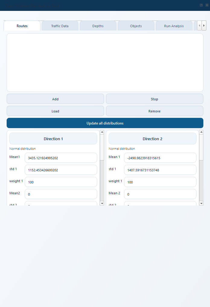
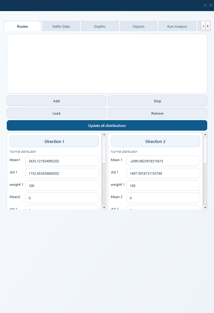
The Routes tab lists every leg of the shipping route. The lateral distribution panel (see Lateral distributions) lives on the same tab, underneath the table.
A route is a polyline split into one or more segments (legs). Each segment has:
Start_Point / End_Point – lon/lat of the two endpoints.
Width – the length (metres) of the dashed tangent line drawn across the leg. The tangent line is also the passage line the AIS query samples when you click Update AIS, so the width bounds which ships are counted. The lateral spread used in the risk calculation itself comes from the distribution panel lower down the same tab.
Tangent (%) – where along the leg the tangent line sits, in percent from the start point. Defaults to 50 (the midpoint). See Moving the tangent line.
Dirs – the two direction labels auto-derived from the segment’s compass bearing (
"North going"/"South going", etc.).bearing – stored compass bearing in degrees.
ai1, ai2 – IWRAP “position check interval” in seconds for directions 1 and 2. Used by the powered-grounding / allision calculations (\(N_{II} = P_c Q \cdot m \cdot \exp(-d/(a_i V))\)). A value of 0 switches Category II off for that direction. On IWRAP export the value goes to the direction’s
grounding_check_time; because IWRAP treats 0 there as “use the global default”, a 0 is exported as a zero leg extension past the waypoint that flow would overshoot instead, and import maps it back the same way.
Click the Segment_Id, Route_Id or Leg_name column header to
sort the table by that column; click again to reverse. Names sort
naturally, so LEG_1_2 comes before LEG_1_10 and LEG_5_12_a
before LEG_5_12_b. The leg selector on the Traffic tab follows the
same order, and so does the saved project.
Editing Width and Tangent (%). One click on a Width or Tangent (%) cell opens it for typing; press Enter to apply (Esc cancels). The map redraws the tangent line and its distribution curves right away. The other columns keep Qt’s usual double-click.
Digitising a route
Click Add Route to start digitising.
Click on the map to set the first waypoint.
Click again to create a leg; each subsequent click adds a segment.
Click Stop Route when done.
Segments are automatically assigned an ID (1, 2, …) and a
default width of 5000 m.
Editing a segment
Select a segment in the route table and edit its geometry directly on the map using QGIS’s standard vertex-editing tools. OMRAT listens to the geometry-change signal and:
Updates the Start_Point / End_Point values in the table,
Recomputes direction labels and stored
bearing,Recomputes
line_length(metres) via UTM projection.
The recomputed values are included in project save and in IWRAP XML export, so map geometry and exported model stay in sync.
Moving the tangent line
By default the tangent line crosses each leg at its midpoint. Where the midpoint is a poor cross-section – close to a junction, a port approach or an anchorage that pollutes the AIS sample – you can slide it along the leg. Its centre always stays on the leg, so the lateral distribution fitted from the AIS passages still refers to the leg centreline.
Three ways to move it, from easiest to most manual:
Type a value in the table. Edit the Tangent (%) cell of the
leg in the route table (0 = start point, 100 = end point) and
press Enter. The dashed line on the map jumps to the new position.
Non-numeric input is reverted to the stored value.
Drag it with the Move tangent button.
Click Move tangent under the route table. OMRAT selects the Tangent Line layer, puts it in edit mode and activates QGIS’s Move Feature tool for you. A message in the QGIS message bar confirms this.
On the map, press the left mouse button on the dashed line you want to move and release it where you want the line to be. (In QGIS 3 Move Feature works with one click to pick up and a second click to drop, not press-and-hold.)
The line snaps back onto its leg at the new position, perpendicular and with the width from the table. Only the movement along the leg counts; dragging sideways or rotating the line has no lasting effect. The Tangent (%) cell updates to match.
Repeat for other legs, then pick the Pan Map tool (hand icon on the QGIS toolbar) to leave the move tool.
Drag it with the QGIS tools yourself. This is what the button does behind the scenes, useful if the toolbar is customised:
In the QGIS Layers panel click Tangent Line so it is the active layer.
If the pencil icon on the layer is grey, click Toggle Editing (the pencil on the Digitizing toolbar) so the layer is editable.
Open the Advanced Digitizing toolbar if it is hidden (View -> Toolbars -> Advanced Digitizing Toolbar) and choose Move Feature. The Vertex Tool on the Digitizing toolbar also works; moving one end of the line moves its centre half as far along the leg.
Click the tangent line, then click where it should go. OMRAT snaps it back onto the leg as above.
Whichever way you use, the position is stored with the leg and saved in the project, and the table and the map always agree. After a move the leg’s traffic is stale until you click Update AIS for that leg; a message-bar hint reminds you. When a leg is split at a crossing, the sub-legs start at 50 % again.
Note
You never need to save the Tangent Line layer’s edits. OMRAT discards the raw drag and redraws the line itself; the layer is a temporary memory layer that is rebuilt from the project file.
Distribution curves on the tangent line
As in IWRAP, every tangent line also shows the leg’s two lateral distributions, drawn to scale on the map. They are always on and are part of the Tangent Line layer, so hiding that layer hides them too.
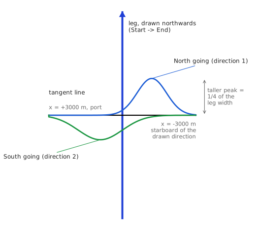
How to read them:
Along the tangent line the curve is the fitted distribution in true scale: the peak sits where the ships actually pass. The curve is the one the calculation uses (up to three normal components plus the uniform part, from the lateral distribution panel), not the raw AIS histogram.
Short dashed ticks mark the powered model’s ray span. Two per direction, in the curve’s colour, at \(\mu \pm 6\sigma\) of the first normal component: that is where the Category I and II rays start and stop (see Ray span and ray count). A tick beyond the end of the tangent line, joined to it by a thin dashed extension, means the rays reach past the drawn lane.
Each direction bulges towards the side its ships sail to. Direction 1 (the drawn direction, Start -> End) bulges towards the leg’s end point and is blue. Direction 2 bulges towards the start point and is green, the same colours as the distribution plot. In the picture the North going ships keep to their starboard side (east) and the South going ships to theirs (west), as in right-hand traffic.
Heights share one scale per leg. The taller of the two peaks is 1/4 of the leg width and both curves have the same area, so a narrow distribution stands out as a tall, thin curve. The height carries no ship count.
The curves span the tangent line. A tail that reaches beyond the leg width is cut off where the tangent line ends.
The curves follow every change: an edit in the distribution panel, a new width or tangent position, Update AIS, Copy traffic, a vertex drag and a project load. A leg without a distribution (all weights 0) has no curves. Dragging a curve does nothing; it snaps back.
In the Layers panel the Tangent Line layer has three legend entries: Tangent line, Lateral distribution, direction 1 (drawn direction) and Lateral distribution, direction 2 (reverse). Restyle them there like any rule-based layer; the style is saved in the project with the other layer styles.
Copying traffic between legs and locking it
When several routes cross each other the validation pass splits them
into many short sub-legs (LEG_5_12_a … LEG_5_12_d). Some of
those sit right in the crossing, where the AIS sample mixes in ships
from the other routes. Rather than accept that sample you can declare
that a sub-leg carries the same traffic as a clean sibling, and protect
that choice from the next AIS refresh.
Click Copy traffic… under the route table.
Pick the source leg (only legs that already hold traffic are listed) and one or more target legs (Ctrl-click for several).
Leave Also copy the lateral distributions ticked to copy the mean / std / weight / uniform / AI parameters and the raw AIS offsets used by the distribution plot. Untick it to copy only the traffic matrices.
Tick Swap directions if the target leg was drawn the opposite way to the source. Direction 1 and 2 are exchanged and the lateral axis is mirrored (means, samples and uniform bounds change sign), because “left of the leg” flips with the drawing direction. For sub-legs of the same original leg leave it unticked.
On OK OMRAT compares the leg bearings (not the direction names: a leg at 44 deg is “North going”, one at 46 deg “East going”, yet they run the same way). If the source’s direction 1 would land on a target direction heading more than 90 deg away, a warning lists those legs with the angle. Swap these legs swaps only them and copies the rest as chosen – the way to copy onto several legs when some are drawn one way and some the other. Copy as chosen ignores the warning; Cancel returns to the dialog.
Leave Lock target legs ticked (default) and press OK.
The dialog does not block QGIS: you can pan and zoom the map while it is open to find the legs you want. Clicking Copy traffic… again brings the open dialog to the front.
Every variable (Frequency, Speed, Draught, heights, beam and the Scaling matrix) is copied per direction, direction 1 to direction 1 and 2 to 2, using the target leg’s own direction labels. If a target is already locked you are asked before it is overwritten.
AIS lock. The last column of the route table, AIS lock, is a
checkbox. A locked leg is skipped by both the per-leg Update AIS
button (you get a message instead) and the global Update all
distributions pass (skipped legs are listed in the message bar).
The Traffic tab marks locked legs with [locked] in the leg
selector. You can tick or untick the box by hand at any time, for
example to protect a leg whose matrices you edited manually. The
flag and the source leg are saved in the project file.
Unlocking a copy releases it. The lock and the copy belong
together: an unlocked copy is replaced by the leg’s own AIS traffic on
the next Update AIS. So unticking AIS lock on a copied leg also
removes its link to the source leg. The leg label loses copy of ...,
the green Traffic links arrow disappears, and the junctions next to the
leg stop forcing 100 % continuation with the source. The message bar
says which link was removed. The copied numbers stay in the leg until
the next AIS update replaces them; ticking the box again locks those
numbers but does not bring the link back (copy again to restore it). In
the same way, an AIS update that writes a leg, for example a copy made
with Lock target legs unticked, clears that leg’s link.
Action |
Leg label |
What the next Update AIS does |
|---|---|---|
After Copy traffic (locked) |
|
skips the leg; the copy stays |
Untick AIS lock |
|
replaces the copied numbers with the leg’s own AIS traffic |
Tick AIS lock again |
|
skips the leg; whatever it holds now stays |
Locking does not stop the leg’s passages from being counted for the junction transition matrices; those still come from AIS (or your manual edits) as described below.
Moving traffic to another route (suppressing legs)
The AIS data shows where ships sail today. A scenario often asks what happens when a lane can no longer be used. The typical case is a planned wind farm built on top of it: the ships take a detour, and the risk that matters is on the detour (more head-on, overtaking and crossing traffic, and allision or drifting towards the farm).
Suppress leg… handles this. A suppressed leg stays in the project, drawn dashed, but is left out of the calculation, and its ships are moved onto the legs you choose. The total number of ships is unchanged, and Restore leg brings the baseline back at any time.
Tip
Run Copy traffic first. The first time you open Suppress leg…, a warning recommends it and offers to open Copy traffic…. The warning is shown once per computer. Copy the traffic of each route’s cleanest leg onto its other sub-legs (see Copying traffic between legs and locking it). The sub-legs then carry the same traffic and are linked as one route at their junctions. This matters most for the detour route: the moved ships are added to its legs, so they should start from consistent traffic.
Copy, move or suppress together?
Three tools change where a leg’s traffic comes from. Pick the one that says what you mean:
You want to say … |
Use |
What happens to the ships |
|---|---|---|
“Leg X has the same traffic as leg Y” (X’s own AIS sample is polluted by a crossing) |
Copy traffic… |
Y’s traffic is written onto X. Both legs are in the calculation, as they should be for two parts of one route. |
“The ships on leg X sail leg Y instead” |
Suppress leg… with targets |
X is left out; its ships are added to Y. Nothing is duplicated. |
“Leg X carries the same ships as leg Y, and Y is already being moved” |
Suppress together with this leg (on Y) |
X is left out and nothing is moved again. |
Important
Two rules cover every case.
Every leg the moved ships sail gets the full share. A detour made of three legs in a row gets 100 % on each of the three legs. Shares are split only between alternative routes.
One route, one lead. The ships of a route are moved by one leg only, the lead. The other legs of the same route are suppressed together with the lead, without targets of their own.
A quick check for rule 1: draw any line across the detour, from one side to the other. The shares on the legs it cuts add up to 100 %.
Example 1: one leg, a detour in a row
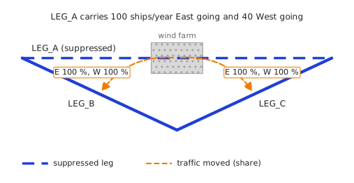
LEG_A crosses the wind farm and carries 100 ships/year East going and
40 West going. After the farm is built the ships sail LEG_B and then
LEG_C. Every ship sails both detour legs, so each gets 100 %.
Pick LEG_A in Suppress leg… and add four rows:
From direction |
To leg |
To direction |
Share (%) |
|---|---|---|---|
East going |
LEG_B |
East going |
100 |
West going |
LEG_B |
West going |
100 |
East going |
LEG_C |
East going |
100 |
West going |
LEG_C |
West going |
100 |
Result in the calculation (assuming LEG_B and LEG_C had 10 ships
each way of their own):
Leg |
Direction |
Before |
After |
|---|---|---|---|
LEG_A |
both |
100 / 40 |
left out |
LEG_B |
East / West |
10 / 10 |
110 / 50 |
LEG_C |
East / West |
10 / 10 |
110 / 50 |
A common mistake is 50 % on each detour leg. That would make only half
the ships sail LEG_B and the other half LEG_C, but both halves
must pass both legs. The cross-section check shows it: a line across the
detour cuts LEG_B only (or LEG_C only), so that leg needs 100 %.
Example 2: the ships split between two routes
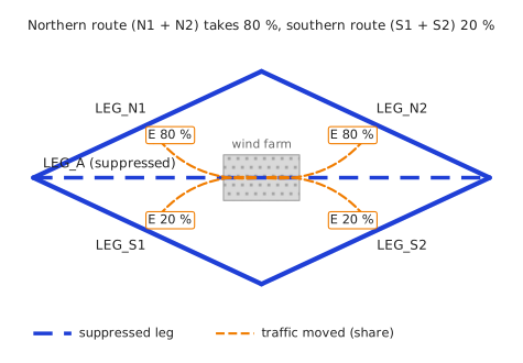
Now there are two detours: a northern one (LEG_N1 then LEG_N2)
taken by 80 % of the ships, and a southern one (LEG_S1 then
LEG_S2) taken by 20 %. Rule 1 still applies inside each route: both
legs of the northern route get 80 %, and both legs of the southern route
get 20 %.
From direction |
To leg |
To direction |
Share (%) |
|---|---|---|---|
East going |
LEG_N1, LEG_N2 |
East going |
80 (one row each) |
East going |
LEG_S1, LEG_S2 |
East going |
20 (one row each) |
West going |
the same four legs |
West going |
80 / 20 as above |
That is eight rows. The shares add up to 200 % per direction, which is correct: a line across the detour cuts one northern and one southern leg, and 80 % + 20 % = 100 %. Result: the northern legs gain 80 East-going ships and the southern legs 20 (and 32 / 8 West going).
The two directions do not have to match. You may send 80 % of the East going ships north but only 50 % of the West going ships, if that is what the traffic does.
Example 3: moving a whole route
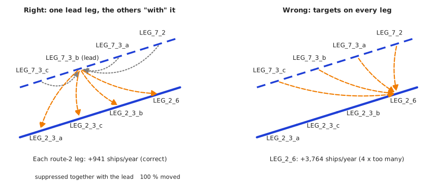
Crossings split a route into several legs. Here route 7 is LEG_7_3_c,
LEG_7_3_b, LEG_7_3_a and LEG_7_2, and all of its ships should
move to route 2 (LEG_2_3_a, LEG_2_3_c, LEG_2_3_b, LEG_2_6).
The four route-7 legs carry the same ships. If each of them had
targets, route 2 would receive those ships four times (right-hand
picture). So:
Before you start, run Copy traffic… along route 2, the detour, so its sub-legs carry the traffic of its cleanest leg (in this project
LEG_2_3_bandLEG_2_3_care locked copies ofLEG_2_3_a).Pick the leg with the cleanest AIS sample as the lead, usually the one furthest from any crossing. Here that is
LEG_7_3_b, with 497 ships/year West going and 444 East going.Open Suppress leg… and pick
LEG_7_3_b.In 1. Suppress together with this leg, tick
LEG_7_3_c,LEG_7_3_aandLEG_7_2.In 2. Where the ships go, add eight rows: both directions, 100 %, onto each of the four route-2 legs (rule 1: route 2 is one detour in a row). To direction is filled in from the leg bearings; check it once.
Click Suppress & move traffic.
The dialog then looks like the picture in the next section.
Result:
Leg |
Before (ships/year) |
After |
|---|---|---|
LEG_7_3_b (lead) |
941 |
left out, ships moved |
LEG_7_3_c, LEG_7_3_a, LEG_7_2 |
(own AIS samples) |
left out, nothing moved |
LEG_2_6 |
7,155 |
8,096 (+941) |
LEG_2_3_b / LEG_2_3_c |
9,873 |
10,814 (+941) |
LEG_2_3_a |
10,741 |
11,682 (+941) |
Things you do not need to do:
Copy the lead’s traffic onto the other route-7 legs to change the result. A leg suppressed together with the lead is never read, so its traffic does not matter. Copying along the detour route (step 1) is what counts.
Unlock the target legs. A lock only stops Update AIS from overwriting a leg’s stored traffic. The move happens during the calculation on a copy of the data, so locked legs (such as copies) are fine as targets. Keep the lead unlocked if you want Update AIS to keep the moved amount current.
Restore leg (+3 with it) on LEG_7_3_b brings the whole of route 7
back. If you open one of the other route-7 legs in the dialog, it tells
you which lead it belongs to.
The dialog, field by field
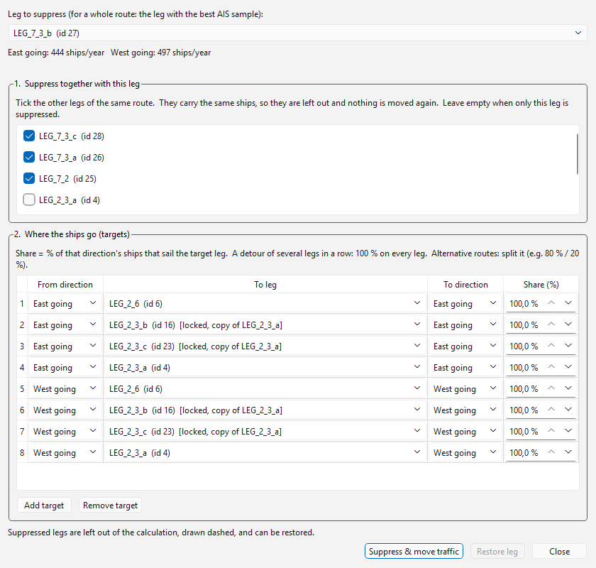
Suppress leg… filled in for Example 3. Top: the lead leg and its ships per direction. Group 1: the rest of route 7, suppressed with it. Group 2: where the ships go.
The dialog does not block QGIS, so you can pan the map while you fill it in. Work through it from the top:
Leg to suppress – the leg whose ships are moved (the lead, for a whole route). Its ships per year per direction are shown underneath. If the leg is already suppressed together with another lead, a note says so.
1. Suppress together with this leg – tick the other legs of the same route (rule 2). Leave it empty when only this leg is suppressed. Legs already suppressed elsewhere are greyed out. A leg cannot be both ticked here and a target.
2. Where the ships go (targets) – one row per target leg and direction (Add target / Remove target):
From direction – which of this leg’s two directions is moved.
To leg – a leg the ships sail instead. Suppressed legs are not offered. The label shows where each leg’s traffic comes from, for example
[locked, copy of LEG_2_3_a].To direction – the direction on the target leg. It is pre-filled with the one pointing the same way, so a target drawn in the opposite direction is handled for you.
Share (%) – the percentage of the From direction ships that sail this target leg.
Suppress & move traffic – stores everything and dashes the legs. If a direction that carries ships has no target, you are asked first, because those ships would then drop out of the calculation.
Restore leg – brings the leg (and the legs suppressed with it) back into the calculation. The targets are kept, so suppressing the leg again restores the same scenario.
What the calculation does
The moved ships are added to the target leg cell by cell (ship type x length). Speed, draught, height and beam become averages weighted by the number of ships.
The target leg keeps its own lateral distribution: the moved ships follow the lane they are moved into.
Traffic scaling (Scaling (%)) is applied first, so the moved ships carry the suppressed leg’s scaling.
Suppressed legs are left out of every model (collisions, powered and drifting grounding / allision, consequence) and out of the junction transition matrices. At a junction, a share that went to a suppressed leg is spread over the remaining legs.
Your project file keeps the original traffic. Only the calculation’s copy is changed, and the project can be saved and reopened with the scenario intact.
Checking the set-up
These tools are easy to lose track of in a busy junction area. Check a scenario in three places.
1. The leg labels. Every leg label in the Copy traffic and Suppress leg dialogs and in the Traffic tab’s leg selector says where the leg’s traffic comes from. With Example 3 set up:
LEG_7_3_b  (id 27)  [suppressed -> LEG_2_6 +3, +3 leg(s) with it]
LEG_7_2  (id 25)  [suppressed with LEG_7_3_b]
LEG_2_3_b  (id 16)  [locked, copy of LEG_2_3_a]
LEG_2_6  (id 6)
2. The map. Press Traffic links under the route table (it stays pressed). A temporary Traffic links layer draws a curved arrow from each leg whose data is used to the leg that uses it. The colours are the same as in the pictures above:
Arrow |
Meaning |
|---|---|
green, solid |
Traffic copied from the source leg ( |
orange, dashed |
Ships moved from a suppressed leg. The label gives the share per
direction, e.g. |
grey, dotted |
A leg suppressed together with a lead (the arrow points to the lead). |
Clicking a leg in the route table highlights it on the map in yellow,
and every leg linked with it in orange – with or without this view, and
also for a leg that has no links (yellow only). In Example 3, clicking
LEG_7_3_b lights up all of route 7 and route 2. The highlight
follows the leg when it is moved and disappears when it is removed.
The layer follows every change and is not saved; press the button again
to remove it.
3. The QGIS log (View -> Panels -> Log Messages, tab OMRAT). Every run lists each move, for example:
Suppressed leg 27 (dir 1): moved 497.0 ships/year (100 %) to leg 6 (dir 1)
Suppressed legs left out of the calculation: 25, 26, 27, 28
dir 1 is the leg’s drawn direction and dir 2 the reverse, the
same as direction 1 / 2 in the lateral distribution panel. A target that does
not exist any more, or that is itself suppressed, is listed as a warning.
Common questions
- My shares add up to more than 100 %. Is that wrong?
No. Shares are per target leg, not per direction. Use the cross-section check instead: a line across the detour should cut legs whose shares add up to 100 %.
- The dialog says “No target is given … those ships are removed”.
On the lead leg this usually means a direction was forgotten: add its rows. If the leg belongs to a route that is already being moved, press Cancel, open the lead leg instead and tick this leg under Suppress together with this leg.
- A detour leg was drawn the other way round.
Nothing to do: To direction is chosen from the bearings. Check the pre-filled value when the detour leg runs almost at right angles to the suppressed leg, where “the same way” is ambiguous.
- Can a target leg be a locked copy?
Yes. See “Things you do not need to do” in Example 3.
- I unlocked a copied leg and it no longer says “copy of …”.
That is intended: unlocking releases the copy (see Copying traffic between legs and locking it). To make it a copy again, run Copy traffic… onto it.
- How do I compare the scenario with today’s traffic?
Run the model with the legs restored (the baseline), suppress them, run again, and compare the two runs on the Compare tab. Restore leg and suppressing again switch between the two without losing the targets.
- What about the IWRAP export?
IWRAP has no suppressed legs, so the export writes the scenario as the calculation sees it. The suppressed legs are left out and their ships are added to the targets. A warning lists every move first, and you can cancel (see the File menu section below).
- What if a suppressed leg is split later?
(For example at a crossing found by Update all distributions.) The first part keeps the targets and the other parts are suppressed together with it, so the ships are still moved once. If a target leg is split, every part gets the same share.
Junctions, crossings and merging
Crossing and merging collisions arise wherever two or more legs meet or cross. OMRAT models the meeting point as a junction carrying a transition matrix that says how traffic from each inbound leg splits across the outbound legs. There is no separate “add crossing” action in the UI:
Snap two leg endpoints together (or share a common waypoint when digitising) and OMRAT registers a junction automatically on save.
Legs that cross in the middle (true X intersections, no shared endpoint) are detected when you click Update all distributions; you’ll be prompted to split each crossing into four sub-legs that meet at a new junction. Splitting also offers to copy the parent legs’ traffic onto the sub-legs.
Open Settings -> Junction transition matrix… to inspect or edit how traffic distributes at each junction. Rows default from geometry (deflection-angle heuristic) and are overwritten by AIS counts when a database is connected: trips (
route_id) that cross one leg’s tangent line towards the junction and another’s away from it (How the AIS counts are made). User edits stick.After Update all distributions the editor opens by itself when at least one junction has three or more legs, that is, where legs merge, diverge or cross. It shows the first such junction and zooms the map to it; the message bar says how many there are. A plain bend (two legs) always continues 100 % and does not open it. The per-leg Update AIS button never opens it.
See Junctions and the transition matrix for the math and the AIS-vs-geometry-vs-user hierarchy.
Connecting and disconnecting legs (Waypoint editor)
Legs that end on the same waypoint form a junction, and the collision model counts crossing, merging and bend encounters there. Open Settings -> Waypoint editor… to change which legs meet at a waypoint without dragging vertices.
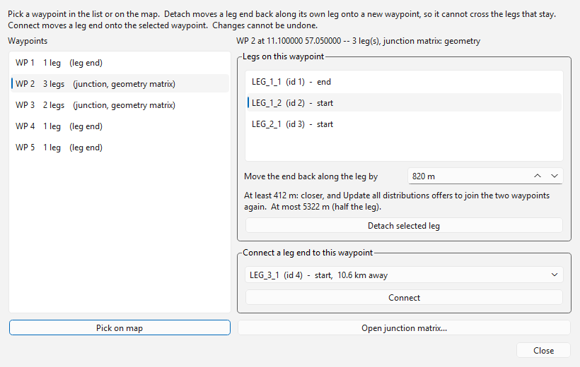
The Waypoint editor. Left: every waypoint with its number of legs. Right: the legs on the selected waypoint, the detach distance and the leg ends that can be connected to it.
Pick a waypoint in the list, or click Pick on map and click it on
the map. While the editor is open a temporary Waypoints (editor)
layer labels every waypoint (WP 12). The selected waypoint is
marked red, its legs yellow, and the leg end chosen under Connect
orange. The layer is removed when the editor closes.
Detach selected leg takes one leg off the waypoint. Its end moves back along its own leg onto a new waypoint, and the other legs stay where they are. The shortened leg is part of the old one, so it cannot cross the legs that remain on the waypoint, or any leg the old leg did not already cross. A blue cross on the map shows where the end will go. The distance has limits:
At least the close-waypoint threshold, 5 % of the shortest leg involved. Any closer and Update all distributions would offer to join the two waypoints again (Junctions and the transition matrix). The suggested value is twice the threshold.
At most half the leg.
A leg that is alone on its waypoint has nothing to detach from.
Connect moves the chosen leg end onto the selected waypoint. The list holds every leg end that is not on the waypoint already, nearest first. Only that one leg moves: other legs on its old waypoint stay put. If the moved leg would cross other legs, the confirmation says which ones, and you are asked to split them right after the move (see Junctions and the transition matrix). The same question comes when you drag a leg end across other legs on the map. To join a leg to the middle of another leg, move a vertex of that leg there first so that it gets a waypoint.
Both actions ask Are you sure? and cannot be undone (save the project first if you want a way back). Afterwards:
the leg, its tangent line and its route-table row follow at once;
AIS transition counts at the junctions the leg touches are reset to geometry, so the next Update AIS counts them again. The leg’s passage line moves with the leg, so run Update AIS on it if its traffic should follow the new geometry;
a junction matrix you edited by hand is kept. A leg that leaves loses its row and column and the other rows are renormalised. A leg that joins gets its geometric row and 0 % in the existing rows; the message bar asks you to check it. Open junction matrix… jumps to the waypoint’s matrix.
Saving the route
File -> Save writes the whole model back to the .omrat file it
was loaded from or last saved to; the file name is shown in the dock
title. For a model that has no file yet it behaves like Save
as…, which always asks for a file name (pre-filled with the current
one, so “save a copy next to it” is a two-click job). Clear model
forgets the file, so the next Save asks again.
The .omrat snapshot that Run Model writes next to each run is
read-only on purpose, so it remains a faithful record of that run. If
you load such a snapshot and press Save, the read-only flag is
cleared and the snapshot is overwritten; use Save as… to keep it
and continue in a new file. The suggested name is then the snapshot’s
stem without the run timestamp (test14_20260827_232733.omrat
becomes test14.omrat).
Closing the OMRAT dock with unsaved changes brings up a prompt with Save, Save as…, Don’t save and Cancel. Cancel, or cancelling the file dialog behind Save as, keeps the dock open. Once the dock closes, all OMRAT layers (legs, tangent lines, depths, structures, drift corridors and result layers) are removed from the QGIS project together with the model; reopen OMRAT and use Load to continue from the saved file.
Layer styling
OMRAT’s layers are memory layers rebuilt from the project file, so a
QGIS project (.qgz) does not keep them. Instead the QGIS style of
each layer type is saved inside the .omrat file when you press
Save and re-applied on Load: legs, the tangent lines, the depth layer
and the structures. Change colours, widths or labels in the QGIS
Layers panel as usual; the style of the first leg (or structure)
layer is used for all legs (structures). A leg drawn after Load picks
up the stored style too. A style change counts as an unsaved change.
Two limits: the depth layer’s automatic colour ramp is re-applied when depth intervals are edited, and result layers from Run Model are not covered.
The on-canvas leg layers in the QGIS Layers panel are memory layers and disappear when you close QGIS. The persistent source of truth is the project file: File -> Save .omrat writes the route (start / end / width / dirs / bearing) plus traffic / depths / objects / distributions to a single JSON file. File -> Open .omrat rebuilds the leg layers from that JSON, so there is no separate “save layer” step.
What flows downstream
Field |
Used by |
|---|---|
|
Every accident type (leg geometry). |
|
Drifting base exposure, ship-ship collision candidate count. |
|
Powered grounding + allision (\(\exp(-d/(a_i V))\)). |
|
Crossing-collision geometry to detect leg pairs that share a waypoint. |
Traffic Data tab
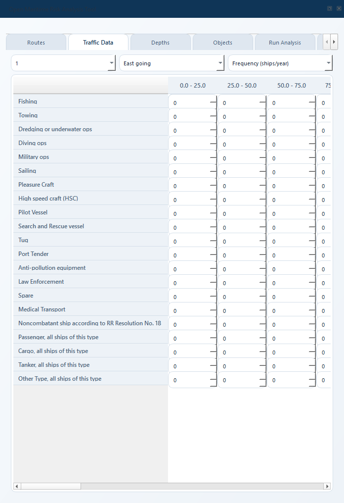
The Traffic Data tab. Matrix rows are ship types, columns are LOA (length) bins.
Every segment, in every direction, has its own traffic matrix. Select a segment and direction using the first two dropdowns at the top, then use the third to pick which variable to edit: Frequency (ships/year), Speed (knots), Draught (meters), Ship heights (meters) or Scaling (%).
Note
Ship Beam (meters) is a sixth variable that is stored per cell
and populated by the AIS refresh, but it is deliberately not
offered in the dropdown – there is no way to edit it by hand. It
is consumed by the ship-ship collision model, which uses it for
the collision width \(B_{ij}\) in the head-on / overtaking
geometric probability and for the collision diameter
\(D_{ij}\) in the
crossing and bend formulas. When a cell has no AIS observation,
the model falls back to an L/B ratio estimate from the LOA bin
midpoint (ShipCollisionModel.estimate_beam), so a hand-entered
project still gets sensible beams.
Editing, and copying to and from Excel
The cells are plain text, like a spreadsheet: click a cell and type,
or double-click to edit. Numbers are shown with your system’s decimal
separator (12,5 on a Swedish Windows, 12.5 on an English one),
and either separator is accepted when you type or paste.
Select – drag over cells, Shift-click / Ctrl-click to extend, click a row or column header for the whole row or column, and the top-left corner button (or Ctrl+A) for everything.
Copy – press Ctrl+C (or right-click Copy). Paste into Excel with Ctrl+V; the numbers arrive as numbers. The Total row and column are not copied.
Copy table with headers (right-click) – the whole matrix with the ship-type and length labels, plus a corner cell naming the leg, direction and variable.
Paste – select the top-left cell and press Ctrl+V. A block copied with headers always lands at the top-left of the table, so you can copy with headers, edit in Excel and paste the whole range back. One copied value pasted onto a selection fills every selected cell. Cells outside the table are ignored, and a cell that is not a number >= 0 keeps its old value. The message bar reports how many cells were pasted and how many of them changed – pasting back an unedited copy says
0 changed.Delete clears the selected cells:
0ships/year for Frequency,100for Scaling, and “no observation” for Speed, Draught and heights.
A blank cell under Speed, Draught or heights means the AIS refresh saw
no ships there (stored as inf); type a value to set one. Cells you
do not change keep their stored value exactly – the table shows two
decimals, but the full value is kept.
Matrix shape
Rows – ship types (configurable under Settings -> Ship Categories; defaults to the 21 IMO types used by IWRAP).
Columns – LOA bins (also configurable; defaults to 15 bins from <50 m to >350 m).
Variables
Variable |
Units |
Used by |
|---|---|---|
Frequency (ships/year) |
ships/year |
Every accident type (exposure). |
Speed (knots) |
knots |
Powered grounding/allision, head-on + overtaking + crossing collisions, drifting exposure. |
Draught (meters) |
m |
Powered grounding depth binning, drifting grounding filter. |
Ship heights (meters) |
m |
Powered allision (clearance check: short ships pass under high structures). |
Ship Beam (meters) |
m |
Ship-ship collision geometry. |
Scaling (%) |
percent |
Per-cell frequency multiplier applied just before risk
integration. |
Scaling traffic up or down
The Traffic Data tab has an easy option for bumping all (or some) of the traffic up or down by a percentage – useful for “what if the forecast goes up 30 %?” sensitivities without editing every cell.
All scaling controls live in a Traffic scaling group box to the left of the matrix. The box is collapsible and starts collapsed so the matrix gets the full width on first open – tick its title checkbox to expand the controls, untick again to fold them away.
Global scaling [%] spinbox inside the group is the master multiplier.
130means every ticked ship-type row gets its Scaling (%) cells set to 130, so \(Q_{effective} = Q \cdot 1.30\) for those rows.Follow global per ship type is the list of checkboxes below the spinbox – one per ship type. Tick (default) = “follow the global”; untick = “leave this row’s values alone”. Use it to exclude e.g. passenger traffic from a cargo-forecast bump.
Switch the variable dropdown to
Scaling (%)to see and edit the per-cell values directly. Typing a value into a cell auto-unticks that ship-type row – the typed number is treated as your explicit override and survives future global changes.Reset all to 100 % clears every override: all checkboxes re-tick, the global snaps to
100, every cell goes back to100.
The scaling matrix is per-leg / per-direction, but the global
broadcast covers every leg + direction at once. AIS refresh and
IWRAP import only overwrite Frequency – never Scaling – so a saved
+30 % survives every traffic update.
Importing from AIS
If you have access to an AIS database:
Settings -> AIS connection settings – enter host, port, database, schema, user, password.
Select a segment in the route table.
Click Update AIS. The plugin queries the database for every vessel passage that crossed the segment’s buffer and populates the traffic table automatically.
The query time is shown in the QGIS log panel.
Note
No AIS database yet? See Database setup and AIS ingestion for the end-to-end guide: standing up the PostGIS schema, ingesting raw NMEA / CSV files through the Database setup wizard, and verifying the tables before clicking Update AIS in OMRAT.
Custom ship type mapping
The AIS type code a ship broadcasts is not always the category you
want it in. Settings -> Ship type mapping… lets you keep a
per-vessel override in the AIS database (the connection from AIS
connection settings is used): enter the schema the table should
live in (the table name defaults to ship_type_map), click
Import CSV…, tick Use the custom ship type mapping and
Save. The dialog previews the table and Export CSV… writes
it back out for editing. The CSV needs an mmsi and/or imo column and a
ship_type column holding the OMRAT category index (0-20), an AIS
type code (30-89) or a name such as Tanker, Cargo or
Passenger; an optional note column is stored as is. OMRAT
creates the table when missing and replaces its rows on every import.
On the next Update AIS each passing ship is classified as: IMO match, else MMSI match, else the external vessel lookup’s ship type column, else the broadcast AIS code. Legs already fetched keep their old categories until you refresh them, so run Update all distributions after changing the mapping.
Depths tab
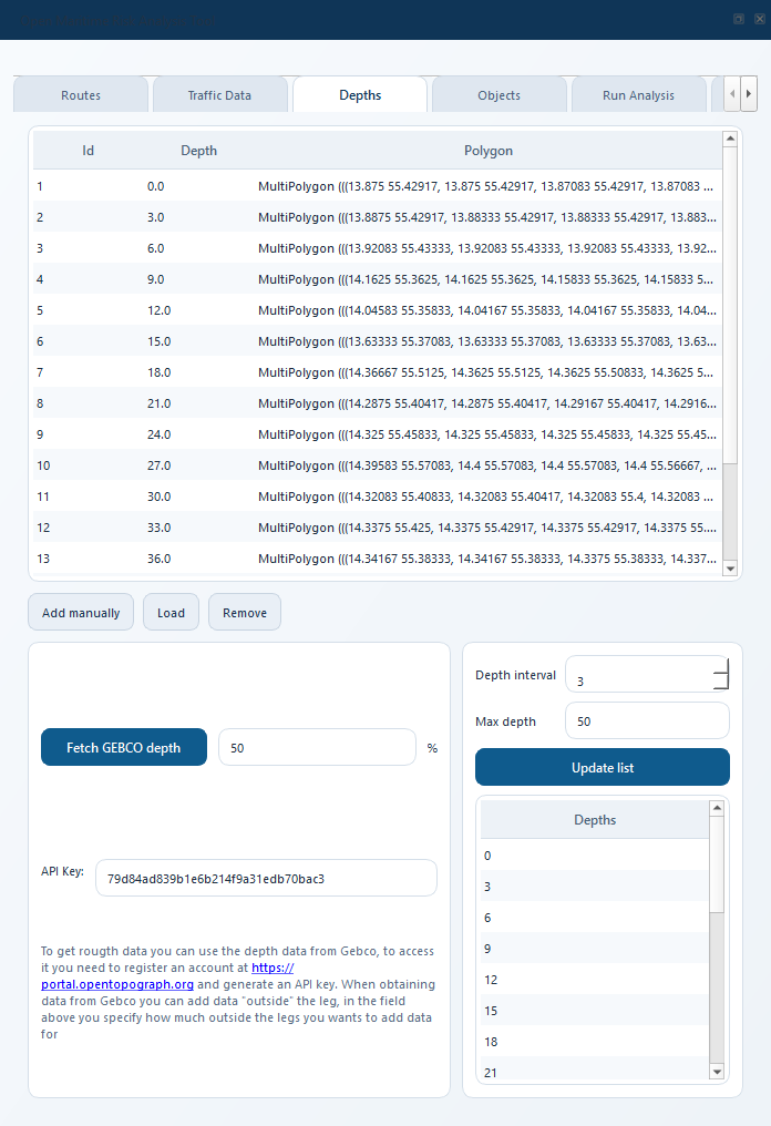
The Depths tab. One row per depth polygon.
Each row has:
id – a short label (auto-generated
d1… or user-set).depth – the water depth at this polygon (metres below chart datum).
Polygon – the WKT geometry, in lon/lat (EPSG:4326).
Adding depths
Three ways:
Add manually – enter a depth value, draw a polygon on the map.
Load – pick a polygon layer; OMRAT imports every polygon and uses the
depthattribute (or the first numeric attribute) as the depth value.Remove – delete the selected row.
Fetch GEBCO depth – requires an OpenTopography API key, pasted into the API Key field on this same tab (not in Settings). Enter the bounding box (Lower-left / Upper-right lat/lon), a Max depth and a Depth interval, click Update list to preview the contour levels, then fetch. The plugin downloads GEBCO bathymetry and vectorises it into depth polygons at those depths.
How depths drive the calculation
Drifting grounding: a polygon’s depth is compared against each ship’s draught. Only polygons shallower than the ship’s draught are grounding hazards for that ship.
Drifting anchoring: a polygon is an anchoring zone if its depth is less than
anchor_d * draught(configurable under Drift settings).Powered grounding: two categories. A shallow polygon inside the leg’s lateral spread is a Category-I hazard (\(N_I = P_{c,I} Q m\), no distance term); the shallowest depth encountered along a ray cast past the leg’s bend gives the Category-II contribution (\(N_{II} = P_c Q m \exp(-d/(a_i V))\)).
Objects tab
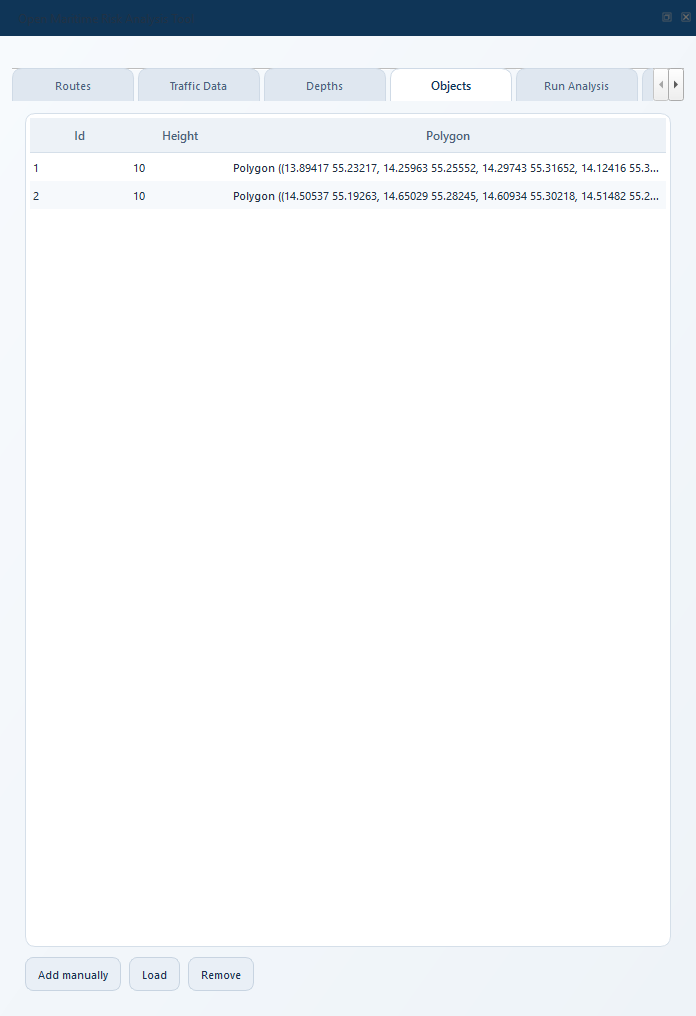
The Objects tab. One row per structure.
Structures are bridges, wind-turbine foundations, platforms, piers. Each row has:
id – label.
height – height of the structure above waterline (metres). Ships shorter than this pass under without colliding.
Polygon – the WKT footprint.
Adding structures
Add manually – enter a height, draw a polygon on the map.
Load – pick a polygon layer with a
heightattribute.Remove – delete the selected row.
How objects drive the calculation
Drifting allision: any ship that drifts into the polygon contributes, regardless of height. There is deliberately no clearance check – a drifting ship has no propulsion and cannot steer away from a structure, so it will impact something on its drift trajectory whether or not its superstructure clears the deck of a bridge. If you want every passing ship counted against an object (e.g. wind-turbine foundations, bridge piers), simply set the object’s
heightto0.Powered allision:
ship_height < object_heightpasses under (no collision) – the powered ship is assumed to clear the structure’s deck. Otherwise the Cat I formula applies to structures inside the leg’s lateral spread and the Cat II formula to structures past the leg’s bend. Setobject_height = 0to disable the clearance check and count every powered ship as well (typical for wind farms and full-height piers).
Lateral distributions
Note
These controls are not a separate tab – they sit in the scrollable panel underneath the route table on the Routes tab.
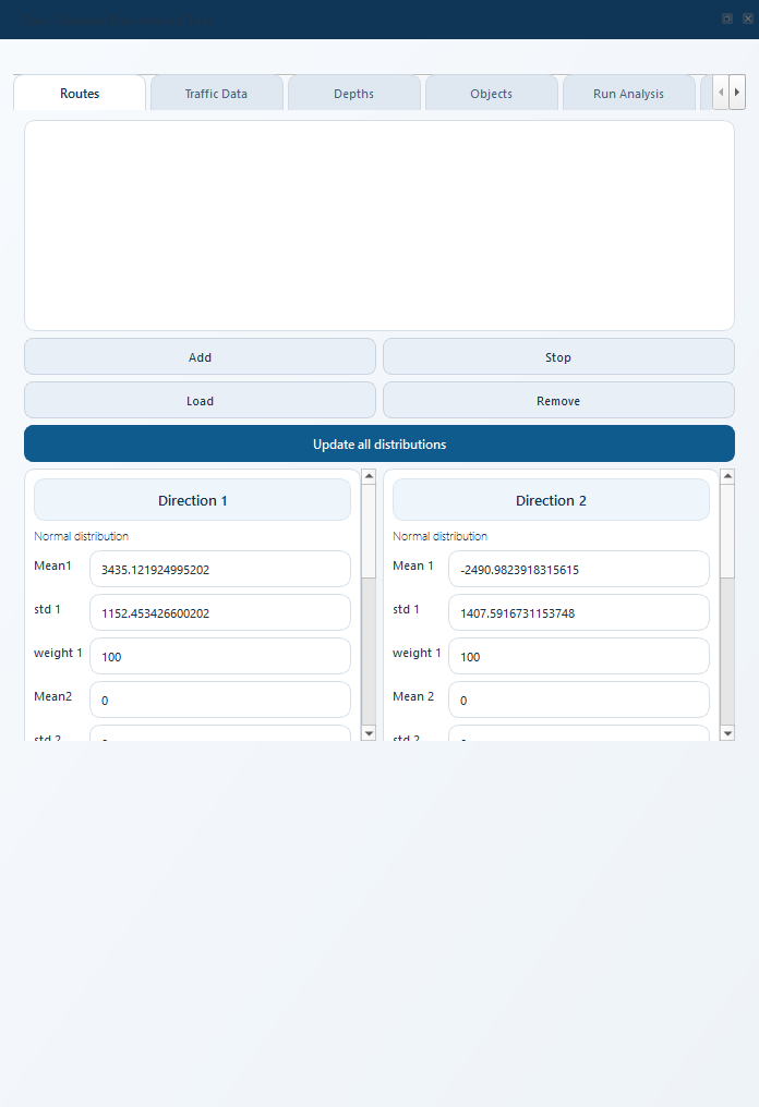
The lateral distribution panel. Two directions per segment; each direction can have up to three Gaussians plus a uniform component.
Per segment, per direction, you can define the lateral traffic distribution – the PDF of where ships are positioned relative to the leg centerline.
Fields
Control |
Meaning |
|---|---|
|
Mean of normal component |
|
Standard deviation of normal component |
|
Weight of normal component |
|
Uniform component bounds, metres. |
|
Weight of the uniform component. |
The plot at the bottom of the tab shows the combined PDF with the sum of (up to 3) normals + 1 uniform.
Why this matters
The lateral distribution enters the calculations in three places:
Powered grounding / allision – defines the “lateral spread” of rays cast across the leg (\(N_\mathrm{rays} = 500\) rays at
mean +/- 4 std).Ship-ship collisions – defines \((\mu, \sigma)\) of each direction for the Gaussian-overlap probability.
Drifting – defines the corridor width (
5 * sigma) and feeds the analytical probability-hole integral.
A segment with zero weights produces zero ship-ship collisions on that direction pair, and a zero-width corridor for drifting – both silent failures. Always check the plot.
Drift Analysis tab
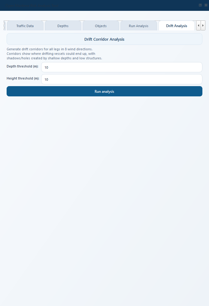
The Drift Analysis tab produces a visual drift-corridor layer.
This tab does not compute the risk – it draws drift corridors for visual inspection. Use it to sanity-check whether the corridors actually reach the obstacles you expect them to hit.
Fields
Depth threshold – hide depth polygons shallower than this (so the corridor isn’t cluttered by the near-shore bathymetry).
Height threshold – same for structures.
Run analysis – kicks off
DriftCorridorTaskin a background thread.
Output
Per leg, per wind-rose direction, a polygon layer is added to the map showing where a drifting ship from that leg in that direction could reach, minus the footprints of any obstacles it would ground or collide on.
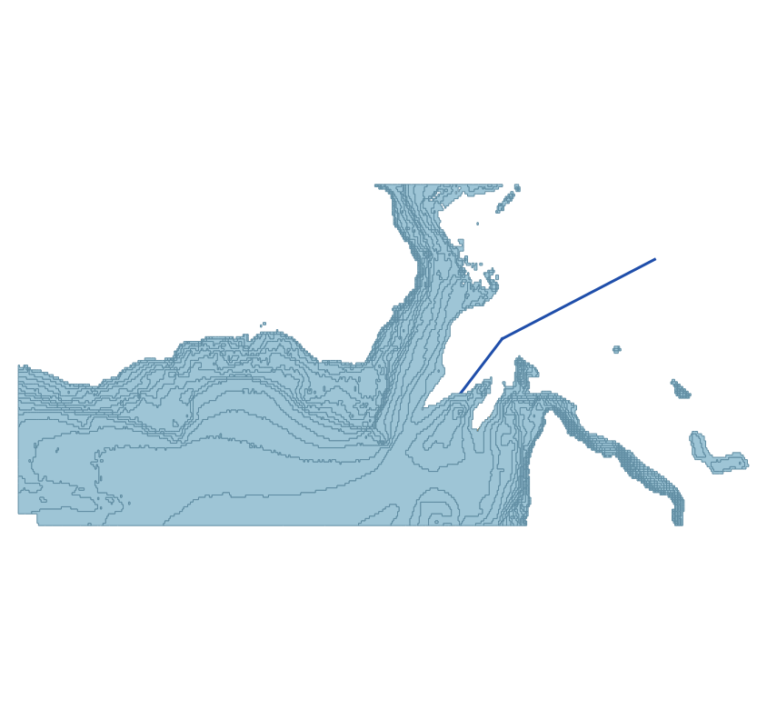
Drift corridors around a leg, coloured by direction. The darker regions are where the ship has already grounded on a shallower polygon closer to the leg.
Run Analysis tab
Note
Older reference material calls this the “Results” tab. It is the same tab; the widget label is Run Analysis.
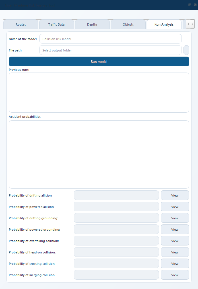
The Run Analysis tab.
Fill in Name of the model and File path (the ... button
opens a folder picker), then click Run model. The button stays
disabled until both are set. It kicks off a
CalculationTask that runs the
drifting, ship-ship collision, powered grounding and powered allision
models in sequence, followed by the oil-spill consequence step. The
task runs in the background so QGIS stays responsive.
Calculation matrix… (right of Run model) picks the model parts a run calculates: Drifting (drifting allision and grounding), Ship-ship collisions (all five types), Powered grounding and Powered allision. Use it to re-run only what a change affects – after moving a wind-farm structure, for example, tick only Drifting and Powered allision. A part that is not ticked is left out of the run, not counted as zero:
its rows in the result table are blank (a calculated zero shows
0);the Markdown report starts with a Partial run line naming the skipped parts, and the GeoPackage and JSON sidecars hold only the calculated parts;
its columns in the run history stay empty, so View on a skipped row tells you to pick a run that includes it;
the oil-spill consequence step uses the calculated parts only.
While parts are left out the button reads Run model (2 of 4 parts) and its tooltip lists them. The selection lasts for the QGIS session.
Results land in two tables: Accident probabilities (one row per accident type, with a View drill-down button) and Catastrophe-level exceedance (events/year). Previous runs above them lists every run in the history; select one and click Add selected run results to map to load its GeoPackage.
Below the nine accident rows the table carries three bold summary rows: All grounding (drifting + powered grounding), All allision (drifting + powered allision) and All collisions (the five ship-ship types). They recompute whenever the rows above change and get their own probability / delta cells when previous runs are compared.
The Show as selector to the right of the table caption switches the
presentation between Frequency (per year) – the annual accident
frequency in scientific notation – and Years between incidents,
i.e. the return period 1 / frequency. The choice applies to the
accident table, its summary rows, the per-run comparison columns and
the catastrophe-exceedance table below, and is remembered between
sessions. Only the presentation changes: the stored totals, the run
history and the Δ % columns are always computed from the frequency.
A zero frequency shows as ∞ in years mode.
The View button on a ship-ship collision row opens a per-leg (or
per-leg-pair) table with the absolute probability and a % of total
column, i.e. each leg’s share of that accident type. The drifting and
powered View dialogs list their legs the same way – route-table
names (LEG_6_1_b East going) and a % of total column – next
to their figures (see Visualization).
Result fields
All values are annual accident frequencies (expected events per
year). They appear in scientific notation (1.148e-01 means 0.1148
events/year or roughly one event every 9 years).
Field |
Meaning |
|---|---|
LEPDriftAllision |
Drifting + hitting a structure. |
LEPDriftingGrounding |
Drifting + running aground on a depth polygon. |
LEPPoweredGrounding |
Under power, failing to turn, hitting a depth polygon. |
LEPPoweredAllision |
Under power, failing to turn, hitting a structure. |
LEPHeadOnCollision |
Two ships on the same leg in opposite directions. |
LEPOvertakingCollision |
Same leg, same direction, different speeds. |
LEPCrossingCollision |
Two legs sharing a waypoint and meeting at more than 30 degrees. |
LEPMergingCollision |
Two legs sharing a waypoint and meeting at 30 degrees or less – streams converging onto nearly the same course. Same equations as crossing, its own causation factor. |
LEPBendCollision |
One leg changing direction at a waypoint: a ship fails to turn and hits traffic that did. |
Note
Changed in v0.14.0
LEPMergingCollision used to be fed the bend total, and
merging itself was summed into crossing. They are now three
distinct rows. See Merging Collisions and the
crossing-formula warning in Ship-Ship Collision Calculations.
The View button next to each row opens a drill-down dialog for the run selected in Previous runs: each leg’s (and direction’s) contribution with its % of total, and – for the drifting and powered rows – a figure of the selected leg with the obstacles it hits. These are useful for locating the leg and the obstacle that dominate the total risk.
Sensitivity analysis
Sensitivity analysis… (below Run model) answers “which inputs
drive the result?”. Every selected parameter is changed one at a
time by -d and +d (default 20 %) around its current value, the
accident totals are recomputed and the parameters are ranked by the
swing they produce in a chosen output.
A full model run takes from half an hour to a few hours on a real project, so the dialog avoids re-running the model wherever it can:
Instant parameters never re-run anything. Causation factors are pure multipliers on their accident type (with the Category I / II split for powered accidents), a change in traffic volume scales drifting and powered totals linearly and ship-ship collisions quadratically, and a change in the volume of one ship type is read first-order exactly from the per-cell breakdowns every model emits. Their ranking appears as soon as the analysis starts.
Computed parameters – ship speed, draught, height and beam, the drift settings (blackout frequency, anchoring probability and depth, drift speed, repair-time distribution), the lateral spread of the legs and the position check interval – re-run only the model phases they can influence. The Model phases re-run column of the parameter tree shows which, and the line under the tree counts the partial runs before you press Run analysis.
Dialog controls:
Perturbation d – the one-at-a-time change in percent.
Baseline – Reuse the results of the last model run (fastest; it assumes the inputs have not changed since that run) or Recompute the baseline first. Only the second option is offered before the first Run model of the session, and after a run that left parts out in the Calculation matrix.
Rank by – the output the ranking uses: all accidents, all grounding / allision / collisions, or a single accident type. It can be switched after the run without recomputing.
Select all / Instant only / Select none – quick selection of the parameter tree. Start with Instant only to get a first ranking in seconds; add the computed parameters for an overnight run.
The analysis runs in the QGIS task manager and can be cancelled; the
parameters finished so far are kept. The Ranking table lists, per
parameter, the output at -d and +d, the Swing (value at
+d minus value at -d, absolute and in percent of the baseline)
and the Elasticity, i.e. the relative change of the output per
relative change of the input: 1 means proportional, 2 quadratic, 0 no
effect. Causation factors therefore always show an elasticity of 1 on
their own accident type; the interesting numbers are the non-linear
ones (repair time, drift speed, lateral spread, check interval) and the
relative size of the swings.
When an output folder is set on the Run Analysis tab the ranking is
written there automatically as <model>_sensitivity_<timestamp>.md
plus a .json with every perturbed total, so a report can be
re-ranked later. Save report… writes the same pair anywhere and
Tornado plot… draws the top parameters as a tornado diagram
(needs matplotlib, which QGIS ships).
Settings menu
Settings are split across seven sub-dialogs accessed from the Settings menu: Drift settings, Ship Categories, Causation Factors, AIS connection settings, Ship type mapping…, Database setup wizard… and Junction transition matrix… (the last one is documented in Junctions and the transition matrix).
Drift settings
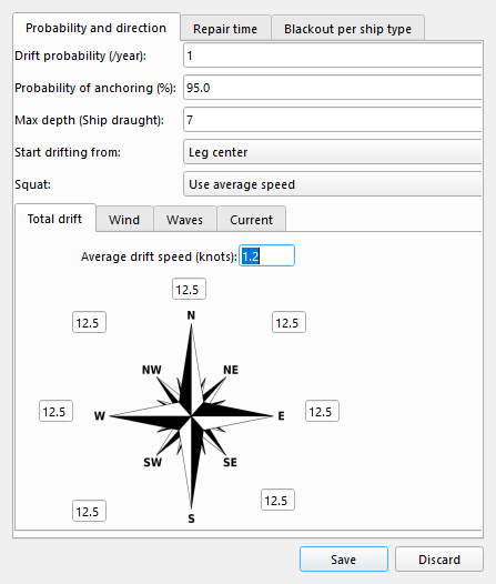
Drift settings dialog.
Field |
Meaning |
|---|---|
|
Blackout rate per ship-year (default 1.0). Multiplied by a
per-type override from |
|
Probability of a successful anchor given the ship is in an anchoring-depth region (default 0.7). |
|
Anchor-depth factor. A ship with draught \(T\) can anchor in water shallower than \(\mathrm{anchor\_d} \cdot T\). |
|
Drift speed in knots. |
Wind rose |
Probability per compass direction, entered as eight percentages that should sum to 100. Type the values freely, then press Check sum: it reports the total next to the S field and, if it is not 100, scales every direction proportionally so the total becomes exactly 100 %. OK applies the same normalisation, so the stored rose always sums to 1. (Earlier versions rewrote the other seven fields as soon as one lost focus, which made entering a whole rose by hand hard.) |
Repair time |
Lognormal / Weibull / Normal CDF parameters for the time-to-repair distribution used to compute \(P_{NR}\). |
All numeric fields in this dialog accept both . and , as the
decimal mark (12,5 and 12.5 are the same value).
Causation factors
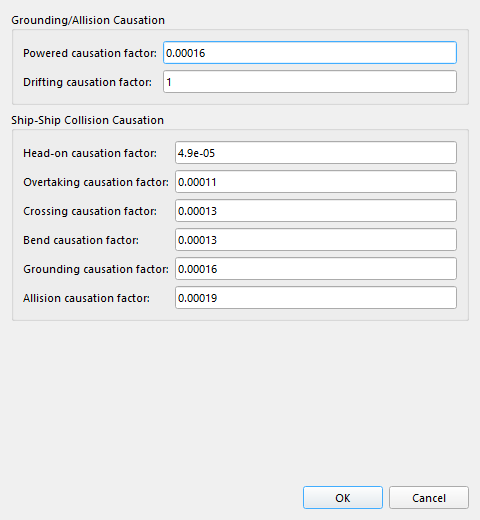
Default values come from Fujii (1974), Pedersen (1995), and the IALA IWRAP manual. See Theory (what is calculated) for the reference table.
Eleven fields: powered, drifting, head-on, overtaking, crossing, merging, bend, grounding and allision (Cat II, missed turn) and grounding and allision Cat I (obstacle already in the lane). The merging factor was added in v0.14.0 and defaults to the crossing value – IWRAP publishes no separate figure for it (see Merging Collisions). The two Cat I factors were added in v0.15.0 together with the Category-I powered model and default to the same figures as their Cat II counterparts, as IWRAP does.
Below the factors sits the Category I start zone group: a checkbox and a percentage (default on, 10 %). With it on, Category I ignores in-lane hits whose first edge crossing lies within that share of the leg, measured from the waypoint the ships come from, for powered grounding and allision alike. It exists because the ships’ lateral positions right after a junction are not yet described by the new leg’s fitted distribution; see The start zone for the reasoning and a worked example. Turn it off to reproduce IWRAP’s plain Category I.
Ship Categories
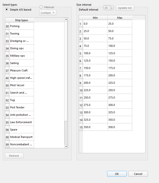
Edit the type names (rows of the traffic matrix) and the LOA bins (columns). Changing these rebuilds the Traffic Data matrix.
AIS connection
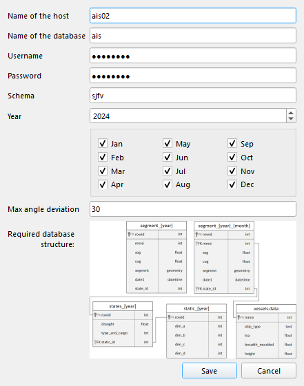
Connection parameters for an AIS PostgreSQL/PostGIS database.
Values are stored in the project file; the password is stored in
plain text, so treat .omrat files as sensitive if you fill
this in.
This dialog only stores credentials. Database setup wizard… on the same menu walks you through creating the database and ingesting data. To stand up the database itself, ingest raw AIS files, and verify that segments are queryable, see Database setup and AIS ingestion.
Ship type mapping
Per-vessel overrides of the AIS ship type, keyed by IMO number or
MMSI. The mapping is a table in the AIS database (schema of your
choice, table ship_type_map by default) holding the OMRAT
category index 0-20 per vessel. The dialog shows a preview of the
table, Import CSV… creates or replaces it from a file with
mmsi and/or imo plus ship_type columns (index, AIS type
code or a name such as Tanker), and Export CSV… writes it
back out for editing. Tick Use the custom ship type mapping and
Save to apply it to the next AIS fetch; an IMO match wins over an
MMSI match, which wins over the external vessel lookup and the
broadcast AIS code. See Custom ship type mapping (IMO / MMSI) for the table
layout and the CSV rules.
Run history (Previous runs)
OMRAT keeps a history of every Run model invocation in two places:
one per-run GeoPackage in the output folder you select, named
<model_name>_<YYYYMMDD_HHMMSS>.gpkg, holding the actual spatial result layers for that run.one lightweight metadata row in the master history database (
omrat_history.sqliteunder the user app-data folder) holding the run name, timestamp, elapsed duration, every total probability, and a pointer (output_dir+output_filename) to the per-run file.
This split keeps the master DB small even after many runs, and gives
you one easy-to-archive .gpkg per run.
The master database location:
Windows:
%APPDATA%\\OMRAT\\omrat_history.sqlite.Linux:
~/.local/share/OMRAT/omrat_history.sqlite.macOS:
~/Library/Application Support/OMRAT/omrat_history.sqlite.
Output folder + Run model gating
Run model is disabled until both Name of the model and
File path are filled in. Use the File path ... button on
the Run Analysis tab to pick a folder – the chosen path is
remembered between sessions. If you trigger the run some other way
with either field empty, a popup names the missing one and nothing
runs.
Projects
The Project name field at the top of the Run Analysis tab names
the project the runs belong to. It is saved in the .omrat file, so
loading the project brings it back, and every run made from the
project is stored under it. Leave it empty and a run is grouped under
the name of its output folder (the last folder of File path) –
the same rule applies to every run recorded before projects existed,
so an existing history is grouped by folder without any work.
Run on the wrong project? Select the runs in Previous runs,
right-click and pick Set project…: choose a project, type a new
name, or clear the text to go back to the output folder name. To
rename a whole project, show it in the Project filter, select all
its rows (Ctrl+A) and use Set project… once.
Naming a run
The Name of the model field on the Run Analysis tab becomes the run’s name AND the filename prefix for all three artefacts written to the output folder:
<name>_<YYYYMMDD_HHMMSS>.gpkg– the result layers.<name>_<YYYYMMDD_HHMMSS>.omrat– a read-only snapshot of the inputs the calculation actually consumed.<name>_results_<YYYYMMDD_HHMMSS>.md– a Markdown report covering every accident type.
Note: result layers are no longer auto-added to the QGIS canvas at the end of a run. Use Add selected run results to map (see below) when you want to look at them.
The Previous runs table
The Previous runs table on the Run Analysis tab shows Name, Main, Date, Duration, Version (the OMRAT version that produced the run) and Project. The Project selector above the table shows one project at a time, with the number of runs in each, or All projects; the Project column only appears for All projects. The selector follows the current project (its project name, else its output folder) until you pick one yourself, and returns to it when a project is loaded or a run finishes. The newest run is selected automatically after a calculation finishes.
For runs recorded before the version was stored, Version is read
once from the run’s .omrat snapshot; it shows a dash when the
snapshot is older than the version stamp or no longer on disk. Selecting rows adds columns to the
Accident probabilities table below:
Single selection – one probability column for that run plus a
Δ %column against the baseline.Multi-selection – one probability +
Δ %column pair per selected run, side by side.
The Main checkbox chooses the baseline: tick exactly one run and
every Δ % column is computed against it (header Δ vs main
(<run name>) %). The choice is remembered between sessions and is
cleared automatically if that run is deleted from the history. With
no main run ticked the baseline is the currently displayed run if
there is one, otherwise the first selected run, and the header says
which (Δ vs current % or Δ vs <run name> %).
Below the table is an Add selected run results to map button. Click it with a single row selected to load that run’s per-run GeoPackage as new layers in the QGIS Layers panel, styled graduated red->green like the live-run output. Multiple selection disables this button – pick one run at a time when loading on the canvas.
The right-click context menu on the table provides:
Add results to map – same as the button (single selection only).
Set project… – move the selected runs to another project (see Projects above).
Delete from history – removes only the row from the master DB; the per-run
.gpkgfile stays on disk so you can keep archived results around if you want.Delete from history + remove .gpkg file – removes both. Asks for confirmation.
Manage previous runs
File -> Manage previous runs… opens the whole history in one window, across all projects: name, project, date, duration, version, output folder and whether the result GeoPackage is still on disk (click a header to sort; newest first by default). The line at the top gives the number of runs, projects and missing result files, and the path of the history file. From there you can:
Set project… – move the selected runs to another project;
Open output folder – of the selected run;
Select runs with missing files – e.g. to delete runs whose results were moved or removed;
Delete from history / Delete + remove .gpkg file – same as the right-click menu of the Previous runs table.
Result-layer attributes
Loading a run onto the canvas adds up to six layers (any layer whose total is zero is skipped):
Layer |
Geometry |
Key attributes |
|---|---|---|
Allision Results (drifting) |
Line |
One feature per boundary edge of each structure.
|
Grounding Results (drifting) |
Line |
Same shape as Allision Results, with |
Powered Allision Results |
Line |
Structure boundary edges again, coloured by the powered
(Cat I + Cat II) probability the ray caster placed on that edge:
|
Powered Grounding Results |
Line |
Same shape, over depth-contour edges. |
Ship-Ship Collision (per leg) |
Line |
|
Ship-Ship Collision (waypoints) |
Point |
|
All layers use the same five-class graduated ramp on
total_edge_probability / combined: green = lowest
contributor, yellow = middle, red = the hotspots that dominate the
total. Line layers are rendered semi-transparent so the
underlying route stays visible.
Compare tab
The Compare tab diffs two finished runs without re-calculating
either. Pick Run A (.omrat) and Run B (.omrat) with the two
... browse buttons – these are the input snapshots each run
writes next to its GeoPackage – then click Compare.
The line under the buttons names the two runs; the results fill five sub-tabs:
Totals – A, B and the absolute and relative difference for the nine accident types, the summary rows (all grounding, all allision, all collisions, all accidents) and, when the runs have a consequence result, the expected oil-spill volume and how often each spill level is exceeded. The values come from the files each run wrote next to its snapshot (
<name>.collision.json,.drifting.json,.powered.json,.consequence.json); the run history only fills in what those files lack. A model part that was not calculated in a run showsn/a, never zero. Above the table: which result files were found, how many differences each tab holds, and the largest single change.Settings & inputs – the settings table lists every scalar under the
drift,pc(causation factors),traffic_scaling,consequenceandship_categoriesblocks that differs, plus per-leg Width. The inputs table lists what decides where accidents happen:legs present in one run only, moved start or end points (with the distance moved) and the Cat II check interval
ai;ships per year per leg and direction, or which other traffic fields differ;
the lateral distribution (mean, std, weight per component, uniform part);
suppressed legs and where their traffic was moved;
junctions present in one run only, the matrix source and the largest change in a transition share;
depth polygons per depth class (count and area of their union, so a layer loaded twice stands out) and structures (height, area).
Legs are matched on id and name. Two different layouts reuse leg ids for unrelated legs, so their legs are listed as present in one run only instead of being diffed against each other.
Breakdown – where the runs differ, item by item: collisions per leg, per waypoint and per leg pair; drifting per leg and per object; powered per leg and direction and per obstacle; oil spill per accident type. Each row has A, B, the change B - A and the item’s share of the summed absolute change in its category. Rows are sorted by the size of the change; Show filters one category and the column headers sort.
Zone – compares only what both runs share: the water within the chosen radius (default 20 km) of the structures of run A and run B, so a run without the park gets the same zone as the run with it. It lists the leg length and traffic work (million ship-km per year) inside the zone, the collisions inside it (head-on and overtaking by the share of each leg inside the zone, crossing, merging and bend by waypoint), collisions per million ship-km, and the allision totals. Use it when two layouts cover different areas: their totals then differ for reasons unrelated to the park. Changing the radius recomputes the table.
Leg lengths – leg-by-leg lengths, so a geometry change shows up immediately.
Why did the collisions change? (More info)
More info (collisions)… under the Totals table explains why each ship-ship collision type changed between A and B. Select an accident row first to open the dialog on that type (any other row opens All collisions).
The inputs that differ between the two snapshots are sorted into groups:
Group |
What belongs to it |
|---|---|
Routing (suppressed legs / moved traffic) |
|
Leg geometry |
start / end points, leg length |
Lateral distributions |
means, standard deviations, weights, uniform part |
Traffic volume |
ships per year, scaling |
Ship properties |
speed, beam, draught, height, length classes |
Junction transition matrices |
the |
Causation factors |
the five collision factors in |
Legs added / removed |
legs present in one run only |
Other leg inputs |
any other leg field the model might read |
The collision model is then re-run with run A’s inputs and each
combination of groups taken from run B. This is quick, because the
ship-ship model is analytic (a few seconds per run). Each group gets
its Shapley value: its effect averaged over every order in which the
groups could be switched from A to B. The values do not depend on an
arbitrary order and add up exactly to B - A. When two groups only
matter together, their joint effect is split between them. With
k differing groups the dialog needs 2^k runs, plus one for run B
itself (B156 with and without the park: four groups, 17 runs, about
half a minute). With more than six groups it averages over 2k
fixed orders, which still adds up exactly. The calculation runs in the
background, and reopening the dialog for the same two files is instant.
The dialog has three parts:
Why – each group’s contribution, its share of the change and a bar (red = increase, blue = decrease). Groups that are identical in A and B are listed underneath. Hover over a group to see what differs.
Largest items – legs (head-on, overtaking, bend) or leg pairs (crossing, merging), each with A, B, the change and its split over the groups. Merge split legs adds up the sub-legs of a split route (
LEG_1_2_a+LEG_1_2_b): moving a split point moves length from one sub-leg to the other, which otherwise looks like two large changes that cancel. Show on map (or a double-click) highlights the selected legs and zooms to them.Findings – plain-language explanations, warnings first:
suppressed legs and where their ships went;
crossing and merging changing in opposite directions because moved traffic meets another flow at a new angle (pairs at 30 degrees or less are merging);
legs whose lateral distribution narrowed or widened, with the effect per leg;
junctions that lost their AIS counts, i.e. fell back to the geometric default after a leg at them was edited. This is usually not part of the scenario;
leg pairs that moved onto, or across, the 30-degree merging / crossing limit;
inputs that differ but do not enter the collision model (
ai, leg width, structures, depth areas). Structures affect collisions only through the route and traffic changes made around them;a warning when the recomputed values differ from the stored results (for example, a run made with an older OMRAT version).
Export to Markdown… writes the summary table, all findings and the largest items for every type to one report.
Note
Only the ship-ship collisions are explained this way. Drifting and powered runs take far too long to repeat for every combination of groups; for those, use the Breakdown sub-tab and the difference layers.
Add both models to QGIS (grouped: A = red, B = blue), right under
the file pickers, creates one layer group per model in the Layers
panel. Each group holds the model’s Depth Areas, Structures,
Legs and Tangent Lines built from the .omrat snapshot, and
– when <name>.gpkg exists next to the snapshot – that run’s
result layers on top. Legs, tangent lines and result layers are
tinted red for A and blue for B. Clear model removes the groups
again.
Add difference layers to QGIS (B - A) answers “where on the map did
the risk move?”. It joins the two runs’ result GeoPackages feature by
feature – obstacle edge for the drifting and powered layers, leg for
collision lines, waypoint for collision points – and adds one
Diff … layer per result type in a group of its own. Each feature
carries p_a, p_b, delta (p_b - p_a in events/year),
ratio, pct_change, delta_share_pct (this feature’s share of
the layer’s total change) and rank (1 = largest absolute change).
The layers are styled on delta: blue = decrease, grey = no change,
red = increase, with class edges at 1, 10, 50 and 100 % of the largest
change. Sort the attribute table on rank to list the movers.
Note
Do not restyle a diff layer on pct_change. Relative change is
dominated by features whose probability is negligible in both runs:
halving a wind-rose direction shows -40 % on thousands of far-away
edges that together move the total by a fraction of a percent, while
the handful of edges that carry the actual increase disappear in the
middle of the ramp. delta and delta_share_pct do not have that
problem.
Tips and best practices
Start with default causation factors. Only adjust if you have local accident data to support different values.
Check the distribution plot on every segment before you trust a result. A zero-weight distribution silently zeroes that segment’s contribution for some accident types.
Use Drift Analysis before Run model on a new project – if corridors don’t reach the obstacles you care about, your result will be near zero and you’ll waste time investigating why.
Result layers colour-code by contribution. Red polygons are your “risk hotspots” and usually the right place to look if the total seems implausibly high.
Keep your repair-time distribution realistic. If it says 90 % of blackouts are repaired in 10 minutes, grounding risk will be near zero regardless of traffic.
Save often. The full result (including the debug-trace breakdown per obstacle, if enabled) is serialised with File -> Save, so a finished run is reproducible.