Quickstart¶

This chapter walks you from a blank QGIS project to a first calculated risk number: how to draw your first leg, bring in depth and object data, fill in the traffic matrix, and read the results.

It is deliberately thin – it only shows the clicks needed to produce a result. Every concept used here (leg, obstacle, traffic cell, drift corridor, causation factor, …) is defined in Concepts, and every tab is documented in detail in User Guide.

Note

A real-world project usually pulls its traffic counts from a PostGIS AIS database via the Update all distributions button – not from manual entry. Setting that database up (schema, raw-NMEA / CSV ingestion, vessel-lookup table, AIS connection settings) is its own multi-step task and is covered end-to-end in Database setup and AIS ingestion. If you’ll need real AIS traffic, read that chapter first so the database is ready before you reach step 6; otherwise you’ll fill the matrix in by hand or come back later.

Tip

In a hurry? Shortcut: start from the example project below loads the bundled example project, which already has traffic, depths and objects filled in – you can jump straight to step 7 and produce a number without an AIS database at all.

Before you start ¶

You need:

QGIS 3.30 or newer (see Installation).
OMRAT installed via the Plugin Manager. On first run the qpip plugin will offer to install the Python dependencies – accept it.

1. Open the plugin ¶

Click the OMRAT icon in the QGIS toolbar. The dock widget docks on the right side of the window.

The dock has a menu bar (File, Settings, Consequence, Help) and a stack of seven tabs: Routes, Traffic Data, Depths, Objects, Run Analysis, Drift Analysis and Compare. The rough workflow is left-to-right.

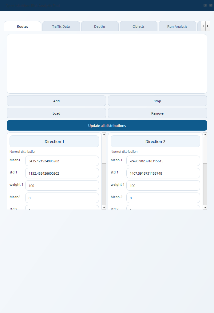
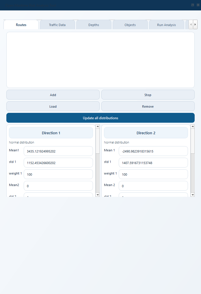
Empty Routes tab, before the first leg is drawn. — Routes tab on a fresh project. `twRouteList` is empty and the distribution panel below it shows zeroed defaults.¶

Empty QGIS canvas with no layers. — The QGIS canvas before any layer is added. Most users begin by adding a basemap (XYZ Tiles -> OpenStreetMap is fine).¶

2. Place legs on the map ¶

A leg is a single straight segment of a route. OMRAT calculates risk per leg, so a curved or branching route is approximated with several short legs joined end to end.

To draw a leg, on the Routes tab:

Set Route (the route ID new legs are assigned to) and Next leg ID if you want something other than the defaults.
Click Add. The cursor turns into a crosshair.
Click the start point on the canvas, then the end point. The leg is added to twRouteList and a blue line appears on the canvas.
Repeat for each leg. Click Stop to leave drawing mode.

Remove deletes the selected leg. Load imports legs from an existing QGIS line layer instead of digitising them by hand.

Routes tab after a single leg has been placed. — The first leg appears in `twRouteList` (Segment 1, Route 1). Adjust **Width** to the width of the corridor in metres (5000 = a 5 km wide corridor).¶

QGIS canvas showing the placed leg as a blue line. — The leg as drawn on the canvas. Two grey “offset” lines mark the width of the corridor.¶

Tip

Endpoints that exactly coincide between legs (within metres, not visually) are treated as shared vertices: dragging one with the QGIS Vertex Tool moves every connected leg’s endpoint together, so a curved route stays connected when you re-route. Shared endpoints also become junctions – see Junctions and the transition matrix.

Below the route table, the same tab hosts the lateral distribution panel (Direction 1 / Direction 2, up to three Gaussians plus a uniform component per direction). The defaults are usable; User Guide explains when to change them.

3. Bring in depth data ¶

Powered grounding and drifting grounding both rely on a depth contour layer. OMRAT consumes depth polygons (one per discrete depth value).

Where to get depth data:

EMODnet Bathymetry (https://emodnet.ec.europa.eu/en/bathymetry) - free 1/16 arc-min DTM for European seas. Download a tile, contour it in QGIS (Raster -> Extraction -> Contour Polygons), then load the resulting polygons into the Depths tab.
GEBCO via OpenTopography - the Depths tab has a built-in downloader that fetches GEBCO depth data directly inside OMRAT. See 3a. Fetching GEBCO depths directly (OpenTopography) below for how to get the free API key required.
Local hydrographic offices - national bathymetry products are usually higher resolution but require a license.
ENCs (Electronic Navigational Charts) - if you have access to S-57/S-101 chart data, the Depth Areas (DEPARE) layer is exactly what OMRAT wants.

Once you have polygons in QGIS, switch to the Depths tab and click Load to import them from a layer. Add manually creates a single empty row you can paste a WKT polygon into, and Remove deletes the selected row.

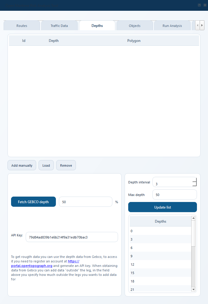
Empty Depths tab. — Depths tab on a fresh project. Each row links one polygon (`Polygon`) to its depth value in metres, positive downwards (`Depth`).¶

3a. Fetching GEBCO depths directly (OpenTopography)¶

OMRAT can download GEBCO bathymetry for your project area and convert it to depth polygons in one click, without leaving QGIS. You need a free OpenTopography API key first.

Step 1 - Create an OpenTopography account

Go to https://portal.opentopography.org and click Create new account (top right). Fill in a username, e-mail address, and password, then confirm your e-mail.

Step 2 - Generate an API key

Log in, then click your username in the top-right corner and choose MyOpenTopo -> My Account. Scroll to the API Access section and click Request API Key. The key is a short alphanumeric string (e.g. abc123def456). Copy it.

Step 3 - Paste the key into OMRAT

In the Depths tab, paste the key into the API Key field. OMRAT saves it automatically between sessions so you only need to do this once.

Step 4 - Enter your bounding box

Fill in the four coordinate boxes:

Lower-left Lat / Lon – the south-west corner of the area you want to download.

Upper-right Lat / Lon – the north-east corner.

A good starting point is to add a small buffer around your routes. You can read off coordinates from the QGIS status bar (shown when you hover over the canvas).

Step 5 - Set depth intervals and fetch

Enter the deepest contour of interest in Max depth and a contour step in Depth interval, both in metres. Click Update list to preview the contour levels in the table on the right, then click Fetch GEBCO depth. OMRAT downloads the GeoTIFF, vectorises it, and adds one row per depth interval to the table automatically.

Note

GEBCO resolution is 15 arc-seconds (~450 m at mid-latitudes). It is appropriate for open-water or offshore risk assessments; for nearshore or port approaches you should use higher-resolution hydrographic charts or ENCs.

4. Define obstacles (objects)¶

Bridges, wind-park footprints, and other surface structures go on the Objects tab. The buttons are the same as on Depths – Load imports a polygon layer, Add manually adds an empty row, Remove deletes the selected one – except that each row carries the structure’s Height in metres above sea level instead of a depth.

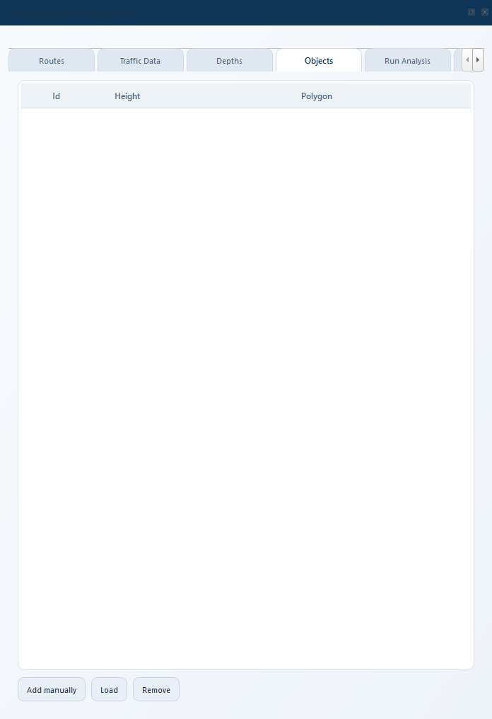
Empty Objects tab. — Objects tab on a fresh project. Powered allision and drifting allision use the polygons listed here.¶

Common sources for object polygons:

OpenStreetMap - bridges, piers and offshore wind farms tagged man_made=* are usually present.
EMODnet Human Activities - offshore platforms, wind-farm layouts.
National marine spatial planning portals.

5. Settings: drift, ship categories, causation, AIS ¶

Open the relevant dialog from the Settings menu at the top of the dock.

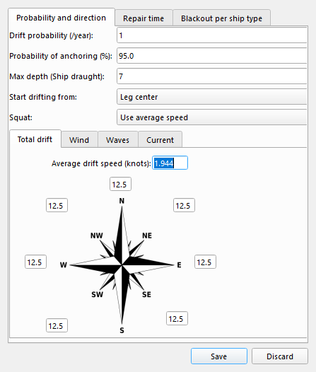
Drift Settings dialog showing the wind-rose. — **Drift settings**. The wind-rose drives drifting risk – start from a uniform 1/8 distribution if you don’t yet have site-specific data, then refine using a local meteorological reanalysis (ERA5, MERRA-2).¶

The other entries on the Settings menu are documented in User Guide:

Ship Categories - the type/size matrix that maps AIS rows to the cells of the traffic table.
Causation Factors - the per-accident-type \(P_c\) values, including a separate Merging causation factor that defaults to the crossing value.
AIS connection settings - host/database/user for the optional AIS Postgres database.
Database setup wizard… - guided creation and ingestion for that database (see Database setup and AIS ingestion).
Junction transition matrix… - how traffic splits between legs at each shared waypoint (see Junctions and the transition matrix).

If you will report oil-spill consequences, the Consequence menu holds the four project-level inputs described in Oil-spill consequence – catastrophe rates.

6. Fill in the traffic matrix ¶

Nothing is calculated without traffic. On the Traffic Data tab, pick a segment and a direction with the two left-hand combo boxes, then use the third to switch between the variables:

Frequency (ships/year) – the number that drives every model.
Speed (knots), Draught (meters), Ship heights (meters).
Scaling (%) – a what-if multiplier applied to Frequency at calculation time; 100 % is a no-op. The Traffic scaling panel underneath drives it globally or per ship type.

Each view is a matrix of ship type (rows) x LOA interval (columns).

If you have an AIS database configured, click Update all distributions on the Routes tab instead: it queries the database, fills Frequency / Speed / Draught / Height for every leg and direction, re-derives the junction transition matrices, and runs the route validation pass (close waypoints and X-intersections). Manually entered Scaling (%) values survive the refresh.

7. Run the model ¶

Switch to the Run Analysis tab and fill in:

Name of the model - a short slug for this scenario.
File path - a folder (use the ... button). Each run writes three files into it:
- <name>_<timestamp>.gpkg - the result layers.
- <name>_<timestamp>.omrat - a snapshot of the inputs (read-only).
- <name>_results_<timestamp>.md - a Markdown report covering every accident type.

Click Run model. The button is greyed out until both fields are set, and a popup spells out which is missing if you click anyway.

The calculation runs as a background QGIS task, so the UI stays responsive. Progress is shown in the QGIS task manager tray at the bottom of the window. The phases run in order:

Drifting model (largest, typically 60–80 % of total time)
Ship-ship collisions
Powered grounding
Powered allision
Oil-spill consequence (if configured)

QGIS task manager showing OMRAT progress — The QGIS task tray shows percent complete and the current phase.¶

8. Read the results ¶

When the run finishes, the Accident probabilities table fills in with one row per accident type, all in expected events per year and scientific notation (1.148e-01 means about one event every 9 years):

Row	Meaning
Drifting allision	Loss of propulsion, then drifting into a structure.
Drifting grounding	Loss of propulsion, then drifting aground.
Powered allision	Under power, failing to turn at a bend, into a structure.
Powered grounding	Under power, failing to turn at a bend, aground.
Overtaking collision	Same leg, same direction, different speeds.
Head-on collision	Same leg, opposite directions.
Crossing collision	Two legs meeting at a waypoint at more than 30 degrees.
Merging collision	Two legs meeting at 30 degrees or less – streams converging onto nearly the same course.
Bend collision	One leg changing direction at a waypoint: a ship fails to turn and hits traffic that did.

The View button on each row opens a drill-down dialog for the run selected in Previous runs, showing per-leg and per-obstacle contributions – the fastest way to find the single obstacle that dominates a total.

If you filled in the Consequence inputs, the Catastrophe-level exceedance (events/year) table below shows the annual rate at which each catastrophe level is exceeded.

9. Inspect the map result layers ¶

Select a row in Previous runs and click Add selected run results to map to load that run’s GeoPackage as styled QGIS layers. (The same action is on the row’s right-click menu, along with the delete options.) Layers that would be empty are skipped, so a missing layer means zero risk of that type:

Layer	Geometry	What it shows
Allision Results	Line	The boundary edges of each structure, coloured by its share of the total drifting-allision probability.
Grounding Results	Line	The boundary edges of each depth contour, coloured by its share of the total drifting-grounding probability.
Powered Allision Results	Line	The same structure edges, coloured by the powered Cat II allision probability (failure-to-turn-at-bend hits).
Powered Grounding Results	Line	Depth-contour edges, coloured by the powered Cat II grounding probability.
Ship-Ship Collision (per leg)	Line	One line per route leg, coloured by `combined` = `head_on` + `overtaking` for that leg.
Ship-Ship Collision (waypoints)	Point	One point at every shared waypoint, coloured by `combined` = `crossing` + `merging` + `bend` there.

All layers share the same green -> yellow -> red graduated ramp: green = lowest contributor, red = the hotspots that dominate the total.

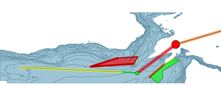
Result map showing drifting, powered and collision layers — A finished run with several layer types visible at once: red structure edges (high drifting-allision contribution), red / yellow line segments along the legs (head-on + overtaking collisions), a red waypoint (crossing / merging / bend collision hotspot), and green features where the contribution is small.¶

Click any feature to open the attribute table. The four obstacle layers carry a per-leg breakdown in leg_<id> columns, so you can trace which leg drove the colour; the collision layers carry the per-mode columns listed above.

Two runs can be compared side by side from the Compare tab – pick two .omrat snapshots and click Compare.

Shortcut: start from the example project ¶

If you just want to see a result without building a project, the source repository ships a complete one at tests/example_data/proj.omrat (4 legs, 17 depth contours, 2 structures, traffic already filled in). If you installed via the Plugin Manager, download it from https://github.com/axelande/OMRAT/tree/main/tests/example_data.

File -> Load in the dock’s menu bar.
Select proj.omrat.
When asked Clear & Load or Merge, choose Clear & Load.

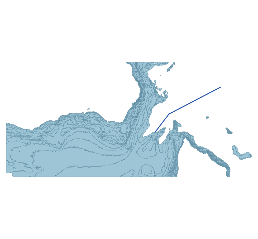
QGIS map canvas after loading the example project — Loaded project: blue route legs on the map, depth polygons in greens/blues, structure polygons in orange.¶

Then skip straight to step 7. Before running, spot-check that the Routes tab lists segments 1–4, that Traffic Data shows non-zero frequencies, that Depths has 17 rows and Objects 2, and set a model name and output folder on Run Analysis.

Note

proj.omrat predates the settings, junction and traffic-scaling blocks, so it loads with defaults for those (scaling 100 %, junctions rebuilt from the geometry). That is expected.

Where to read next ¶

You now have a working run. From here:

Want to understand the numbers? -> Theory (what is calculated) for the big picture, Drifting Risk Calculations for a worked example.
Want a reference for every tab and field? -> User Guide.
Want a glossary of terms? -> Concepts.
Want real AIS traffic? -> Database setup and AIS ingestion.
Want to know what the code did under the hood? -> Code Flow: From “Run model” to Results.

Troubleshooting ¶

The Run model button is greyed out.: Both Name of the model and File path must be filled in on the Run Analysis tab.
All result values are zero.: Check that the Routes, Traffic Data, Depths and Objects tabs all have data – an empty traffic matrix short-circuits the calculation to zero. Then check Settings -> Drift settings: if the blackout rate drift_p is zero, drifting risk is zero.
The calculation runs for more than 10 minutes on a small project.: That is much longer than expected. Open View -> Panels -> Log Messages Panel -> OMRAT and look for warnings. If shapely is missing, qpip’s first-run install may not have completed – see Manual dependency install (fallback).
I want to interrupt the run.: Click the cancel button next to the OMRAT task in the QGIS task tray. The next progress-callback check will abort the calculation.