Powered Grounding and Allision

This chapter describes OMRAT’s calculations for powered grounding and allision – accidents involving ships that are under power but fail to navigate correctly. Two categories are modelled based on Hansen (2008).

Overview

Powered accidents occur when a vessel has operational engines but the crew fails to take appropriate action. This can happen because of:

• Navigation errors

• Equipment malfunction

• Human factors (fatigue, distraction)

• Environmental conditions (poor visibility)

Unlike drifting accidents, powered accidents depend on the lateral traffic distribution relative to obstacles and the probability of course correction after an error.

Current implementation notes:

• Powered grounding uses effective depth bins (by depth contour)

  instead of recomputing geometry for every individual draught value.

• Progress is reported per obstacle-bin step, so long runs show

  meaningful status updates in the task manager.

Grounding pipeline: compute/powered_model.py:417 – run_powered_grounding_model() | Allision pipeline: compute/powered_model.py:458 – run_powered_allision_model() | Exponential decay: compute/basic_equations.py:96 – powered_na()

Category I: Direct Overlap

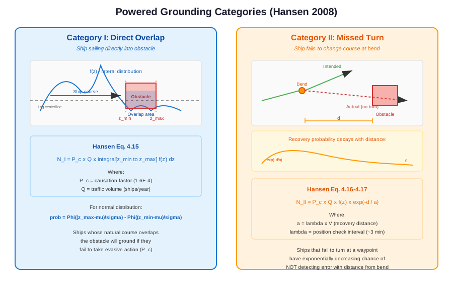
Category I covers ships whose natural course (based on their lateral position in the traffic distribution) takes them directly into an obstacle. These ships are sailing on a heading that overlaps with the obstacle, and will ground/collide unless they take evasive action.

Equation (Hansen Eq. 4.15)

\[N_I = P_C \times Q \times \int_{z_{\min}}^{z_{\max}} f(z) \, dz\]

Where:

• \(P_C\) = causation factor (\(1.6 \times 10^{-4}\) for grounding)

• \(Q\) = traffic volume (ships/year)

• \(f(z)\) = lateral traffic distribution (PDF)

• \(z_{\min}, z_{\max}\) = lateral extent of the obstacle

• The integral represents the fraction of traffic whose course overlaps the obstacle

For a normal distribution, the integral evaluates to:

\[\int_{z_{\min}}^{z_{\max}} f(z) \, dz = \Phi\!\left(\frac{z_{\max} - \mu}{\sigma}\right) - \Phi\!\left(\frac{z_{\min} - \mu}{\sigma}\right)\]

Where \(\Phi\) is the standard normal CDF and \(\mu, \sigma\) are the mean and standard deviation of the lateral position distribution.

compute/basic_equations.py:754 – get_powered_grounding_cat1()

Category I – direct overlap (compute/basic_equations.py)

def get_powered_grounding_cat1(
    Q: float,
    Pc: float,
    prob_in_obstacle: float
) -> float:
    """
    Calculate powered grounding Category I - ships sailing directly into obstacle.

    Category I covers ships that are in the traffic lane that overlaps the obstacle.
    These ships are sailing on a course that would naturally take them into the
    obstacle zone without any course deviation.

    Based on Hansen Eq. 4.15:
    N_I = P_c × Q × prob_in_obstacle

    Where prob_in_obstacle = ∫(z_min to z_max) f_i(z) dz
    (the integral of the traffic distribution over the obstacle extent)

    Parameters
    ----------
    Q : float
        Traffic volume (ships/year)
    Pc : float
        Causation factor - probability that a ship fails to take evasive action
    prob_in_obstacle : float
        Probability of being in obstacle zone. This is the integral of the
        lateral traffic distribution f(z) over the obstacle extent from z_min
        to z_max. Typically computed as Φ((z_max - μ)/σ) - Φ((z_min - μ)/σ)
        for a normal distribution.

    Returns
    -------
    float
        Expected number of Category I powered groundings per year
    """
    return Pc * Q * prob_in_obstacle

Physical Interpretation

Category I accidents are “ships sailing into the obstacle”. Even though the ship has power, the crew may not be paying attention, may not see the obstacle (e.g., submerged reef), or may misjudge the ship’s position. The causation factor \(P_C = 1.6 \times 10^{-4}\) means that roughly 1 in 6,000 geometric encounter candidates results in an actual accident.

Implementation: in-lane ray casting

OMRAT evaluates the integral numerically with the same ray caster as Category II (see Shadow-Aware Ray Casting below), so shadowing and arbitrary polygon shapes come for free:

1. For each leg and direction, cast N_RAYS = 1000 rays parallel to the leg from the waypoint the ships come from, each carrying the mass \(m_i = f(z_i)\,\Delta z\) of its lateral offset.

2. Clip every ray at the leg length. An obstacle past the far waypoint is Category II territory for this leg; an obstacle whose near face lies inside the leg is hit before the turn and counts here. The two categories therefore never score the same water twice.

3. Keep the first obstacle each ray hits. A shoal lying behind another shoal along the leg only receives the rays the nearer one let through.

4. Per obstacle, mass is the sum of intercepted ray masses and

   \[N_I = P_{C,I} \times Q \times \text{mass}\]

   with no distance term – the ship is already on a collision course, and neither its speed nor the position-check interval enters. For grounding the draught filter (depth \(\le\) ship draught) and for allision the clearance check (ship height \(\ge\) structure height) apply exactly as for Category II.

The start zone

Right after the origin waypoint the parallel-ray picture is wrong: the ships are still arriving from the previous leg, and their lateral position is not yet described by this leg’s fitted distribution. An obstacle lying next to a junction would otherwise collect the far tail of the distribution of a leg whose ships never sail there. In the ESCOW case study a wind farm 5 km from a junction received 88 % of its powered allision from the East-going flow of the leg leaving that junction: the park began 2.4σ to starboard of the fitted mean and the 0.8 % tail beyond it, times 10,000 ships a year and the causation factor, gave 1.5e-2 allisions a year, all within the first 8.5 km of a 134 km leg.

Settings > Causation factors > Category I start zone (default on, 10 %) drops every Cat I ray whose first edge crossing lies within the given share of the leg, measured from the waypoint the ships come from. Three consequences follow from the rule being applied per ray:

• An obstacle straddling the line keeps the rays that cross an edge beyond it; those rays are credited to the edge where they leave the start zone.

• The opposite direction is unaffected: its rays start at the far waypoint, so the same obstacle is met at 90-100 % of the leg and still counts (in the example the West-going ships are centred on the other side of the leg and never reach the park in either case).

• Category II is untouched. A ship that misses the turn at the junction and continues straight along the previous leg is still scored by that leg’s Category II.

Switching the setting off reproduces the plain IWRAP-style Category I. The results Markdown states the setting under each powered section, and the Compare tab lists it among the settings differences when two runs disagree.

geometries/get_powered_overlap.py – _compute_cat1_in_lane() | compute/powered_model.py – _iter_hit_probs()

Tip

A wind farm placed alongside a straight leg, well inside its lateral spread, is a pure Category-I case: no bend is involved, so the Category-II model sees nothing. Check the Category I line in the results Markdown when comparing with IWRAP.

Category II: Missed Turn at Bend

Category II covers ships that fail to change course at a waypoint/bend. The ship continues on its original heading instead of turning, and may collide with an obstacle that lies ahead on the original course.

Note

run_powered_grounding_model and run_powered_allision_model compute both categories and report their sum as the powered total; the split is kept in the report under totals['cat1'] / totals['cat2'] and in the Markdown results file. Each category has its own causation factor: pc['grounding'] / pc['allision'] are the Category-II factors (IWRAP p_*_no_turn_causation) and pc['grounding_cat1'] / pc['allision_cat1'] the Category-I ones (IWRAP p_*_causation) – see IWRAP causation-factor mapping. Before v0.15.0 OMRAT computed Category II only.

The probability decreases exponentially with distance from the bend, because the crew has more opportunities to detect and correct the course error the further they travel.

Equation (Hansen Eq. 4.16–4.17)

\[N_{II} = P_C \times Q \times f(z) \times \exp\!\left( -\frac{d}{a} \right)\]

Where:

• \(d\) = distance from the bend to the obstacle (metres)

• \(a = \lambda \times V\) = recovery distance (metres)

• \(\lambda\) = position check interval (minutes, converted to seconds)

• \(V\) = ship speed (m/s)

• \(f(z)\) = probability density at the lateral position where the original heading leads to the obstacle

compute/basic_equations.py:792 – get_powered_grounding_cat2()

Category II – exponential decay (compute/basic_equations.py)

def get_powered_grounding_cat2(
    Q: float,
    Pc: float,
    prob_at_position: float,
    distance_to_obstacle: float,
    position_check_interval: float,
    ship_speed: float
) -> float:
    """
    Calculate powered grounding Category II - ships failing to turn at bend.

    Category II covers ships that fail to change course at a bend/waypoint
    and continue on their original heading towards an obstacle. The probability
    of grounding decreases exponentially with distance from the bend as ships
    have more opportunities to detect and correct their course error.

    Based on Hansen Eq. 4.16-4.17:
    N_II = P_c × Q × f(z) × exp(-d / a)

    Where:
    - d = distance from bend to obstacle (m)
    - λ = position check interval (minutes, converted to seconds)
    - a = λ × V = distance between position checks (recovery distance)
    - f(z) = probability density at the bend position

    The exponential term exp(-d/a) represents the probability that the ship
    has NOT detected its course error before reaching the obstacle.

    Parameters
    ----------
    Q : float
        Traffic volume (ships/year)
    Pc : float
        Causation factor - probability that a ship fails to take evasive action
    prob_at_position : float
        Probability density f(z) at the bend position. This represents the
        likelihood of a ship being at the lateral position where it would
        head towards the obstacle after missing the turn.
    distance_to_obstacle : float
        Distance d from the bend to the obstacle (meters)
    position_check_interval : float
        λ - Position check interval (minutes). Typical value is ~3 minutes.
        This represents how frequently the navigator checks the ship's position.
    ship_speed : float
        Ship speed V (m/s)

    Returns
    -------
    float
        Expected number of Category II powered groundings per year
    """
    # Calculate recovery distance a = λ × V
    recovery_dist = get_recovery_distance(position_check_interval, ship_speed)

    # Avoid division by zero
    if recovery_dist <= 0:
        return 0.0

    # Exponential decay: probability of not detecting course error
    # before reaching obstacle at distance d
    prob_not_recovered = exp(-distance_to_obstacle / recovery_dist)

    return Pc * Q * prob_at_position * prob_not_recovered

Recovery Distance

The recovery distance \(a\) represents the average distance a ship travels between position checks:

\[a = \lambda \times V = (\lambda_{\text{min}} \times 60) \times V\]

Where \(\lambda_{\text{min}}\) is the position check interval in minutes. A typical value is \(\lambda = 3\) minutes, meaning the navigator checks the ship’s position approximately every 3 minutes.

For a ship travelling at 10 knots (~5.1 m/s):

\[a = 3 \times 60 \times 5.1 \approx 920 \text{ m}\]

compute/basic_equations.py:730 – get_recovery_distance()

Exponential Decay

The term \(\exp(-d/a)\) represents the probability that the ship has not detected its course error before reaching the obstacle.

• At \(d = 0\) (obstacle at bend): \(\exp(0) = 1\) (no time to detect)

• At \(d = a\) (one check interval away): \(\exp(-1) \approx 0.37\)

• At \(d = 3a\) (three check intervals): \(\exp(-3) \approx 0.05\)

• At \(d = 5a\) (five check intervals): \(\exp(-5) \approx 0.007\)

This means obstacles close to bends are much more dangerous than obstacles far from bends, because the crew has less time to detect and correct the error.

Physical Interpretation

Category II models the “missed turn” scenario. A ship approaching a waypoint should change course, but some fraction of ships (weighted by \(P_C\)) continue straight. The exponential decay represents the crew’s progressive awareness: at each position check interval, they have a chance to notice they are off course and correct.

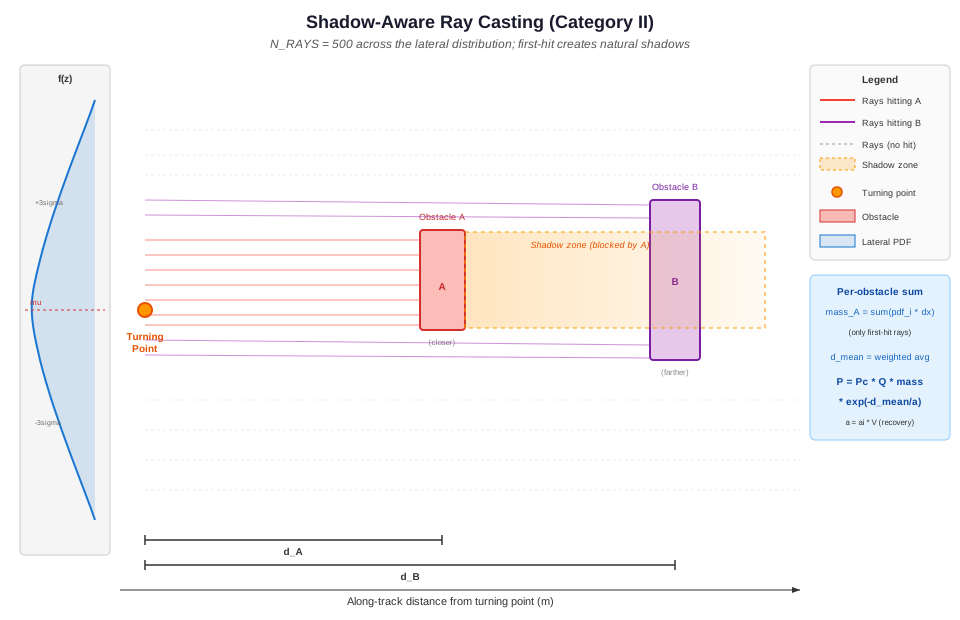
Shadow-Aware Ray Casting

The Category II equations above describe the probability for a single ray from the turning point to a single obstacle. In practice, the lateral traffic distribution means ships may be at any lateral offset when they miss the turn. OMRAT evaluates this by casting 1000 rays across the lateral distribution, from \(\mu - 6\sigma\) to \(\mu + 6\sigma\).

The Algorithm

For each leg and direction (turning point + extension direction):

1. Sample the lateral distribution: Generate N_RAYS = 1000 equally spaced offsets from \(\mu - 6\sigma\) to \(\mu + 6\sigma\) (compute/ray_sampling.py), where \(\mu\) and \(\sigma\) are the lateral distribution parameters.

2. Compute PDF weights: For each offset \(z_i\), evaluate the normal PDF and multiply by the spacing:

   \[m_i = f(z_i) \times \Delta z\]

   This gives the probability mass carried by each ray.

3. Cast each ray: From the turning point offset laterally by \(z_i\), cast a ray in the extension direction (the heading the ship would continue on after missing the turn). The ray extends up to 50 km.

4. First-hit logic: For each ray, find the closest obstacle it intersects. This is the key step – a ray can only hit one obstacle. If obstacle A is closer than obstacle B on a given ray, only A receives that ray’s mass.

5. Accumulate per obstacle: For each obstacle, collect:

   • mass = sum of \(m_i\) for all rays that hit it (first)

   • weighted distance = \(\sum m_i \times d_i\)

   • mean distance = weighted distance / mass

   • probability integral = \(\sum m_i \times \exp(-d_i / a)\)

6. Compute final probability: For each obstacle:

   \[P_{\text{obs}} = P_C \times Q \times \text{mass} \times \exp\!\left(-\frac{d_{\text{mean}}}{a}\right)\]

   Where \(a = \lambda \times V\) is the recovery distance.

Performance Optimization (Depth-Bin Caching)

Powered grounding now groups ships by an effective depth bin:

1. Extract unique depth contour values from depths.

2. Map each ship draught to the deepest contour that is still shallower than or equal to that draught.

3. Run expensive shadow/ray computations once per bin, then reuse results for all ship classes mapped to that bin.

This avoids repeated ray-casting with identical obstacle sets and significantly reduces runtime on projects with many draught entries.

compute/powered_model.py:85 – depth-bin grouping and caching in run_powered_grounding_model() | compute/powered_model.py:114 – per-bin progress updates | compute/powered_model.py:178 – ship draught -> cached bin mapping

geometries/get_powered_overlap.py:415 – _compute_cat2_with_shadows()

Shadow Effect

The first-hit logic naturally creates shadows. When a closer obstacle intercepts a set of rays, those rays never reach any obstacle behind it. The farther obstacle only receives rays that pass around the closer one.

Lateral offset (z)
|
|  miss  miss  miss                 miss  miss
|   .     .     .                     .     .
|    .    .    .          SHADOW        .    .
|     .   .   .    +---------+------+   .   .
|   hit-A hit-A    | Obs A   | (blocked)|   .
|     .   .   .    +---------+------+   .   .
|    .    .    .          SHADOW        .    .
|   .     .     .                     .     .
|  hit-B hit-B hit-B               hit-B hit-B
+---------------------------------------------------> distance

This approach differs from drifting risk, where shadows are created by geometric subtraction of corridor polygons. In the powered model, shadows emerge from the ray-casting itself – no explicit shadow geometry is needed.

Mass conservation: The sum of masses across all obstacles plus the “miss” mass (rays that hit nothing) equals 1.0 (within numerical precision). Each ray’s mass is assigned to exactly one obstacle or none, so there is no double-counting.

The View dialog (see Visualization below) makes this visible: the lateral distribution strip of each Cat I / Cat II panel is filled with the colour of the obstacle each ray hits first, and the rays stop at that obstacle.

Draft Filtering for Grounding

For powered grounding, not all depth areas are hazardous. A depth area is only a grounding risk if the water is shallower than the ship’s draught:

\[\text{Hazard if:} \quad \text{depth} \leq T_{\text{ship}}\]

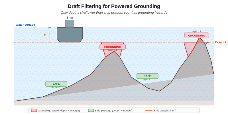
Where \(T_{\text{ship}}\) is the ship’s draught in metres.

Since different ship types have different draughts, the set of obstacles varies per ship type. A large tanker with \(T = 15\) m faces more grounding hazards than a small ferry with \(T = 4\) m.

To avoid running the expensive ray-casting computation once per ship type, OMRAT groups ships by unique draught values:

1. Collect all unique draughts from the traffic data

2. For each unique draught, filter depth areas to those \(\leq T\) and build the obstacle list

3. Run the shadow-aware ray casting once per draught bracket

4. When summing per-ship-type contributions, look up the pre-computed results for the closest matching draught bracket

For powered allision (hitting structures above water), draft filtering does not apply – all objects are obstacles regardless of ship draught.

compute/powered_model.py:215 – _collect_draught_set()

Computation Pipeline

The full powered risk computation is orchestrated by powered_model.py, which provides two methods: run_powered_grounding_model() and run_powered_allision_model().

Grounding Pipeline

1. Build equirectangular projector from first segment
2. Collect all unique draughts from traffic data
3. For each unique draught:
   a. Filter depth areas to those <= draught
   b. Build projected obstacle list
   c. Run _run_all_computations():
      For each (leg, direction):
        - Determine turning point and extension direction
        - Cat II: cast 1000 rays from the turning point onwards
        - Cat I:  cast 1000 rays along the leg, clipped at its length
        - First-hit logic assigns each ray to nearest obstacle
        - Accumulate mass and mean distance per obstacle and category
4. For each (leg, direction, LOA class, ship type):
   a. Get ship frequency Q, speed V, draught T, check interval ai
   b. Look up shadow results for closest draught bracket
   c. For each obstacle hit:
      Cat II: total += Pc_II * Q * mass * exp(-d_mean / (ai * V))
      Cat I:  total += Pc_I  * Q * mass

Allision Pipeline

The allision pipeline is simpler because no draft filtering is needed:

1. Build equirectangular projector from first segment
2. Build projected obstacle list (all objects, ignore depths)
3. Run _run_all_computations() once for all obstacles (Cat I + II)
4. For each (leg, direction, LOA class, ship type):
   a. Get ship frequency Q, speed V, check interval ai, ship height
   b. Skip obstacles the ship clears (ship height < structure height)
   c. For each obstacle hit:
      Cat II: total += Pc_II * Q * mass * exp(-d_mean / (ai * V))
      Cat I:  total += Pc_I  * Q * mass

Per-Ship-Type Parameters

The final summation loops over every ship type in the traffic data. Key parameters that vary per ship type:

Parameter	Symbol	Effect
Traffic frequency	\(Q\) (ships/year)	Linear scaling of risk
Ship speed	\(V\) (m/s)	Affects recovery distance \(a = \lambda \times V\)
Ship draught	\(T\) (m)	Determines which depths are hazards (grounding only)
Position check interval	\(\lambda\) (seconds)	Affects recovery distance; set per segment direction

Faster ships have a longer recovery distance, which means the exponential decay is gentler – obstacles far from the bend are relatively more dangerous for fast ships. Conversely, slow ships have a short recovery distance, so the exponential drops off quickly.

compute/powered_model.py:417 – run_powered_grounding_model() | compute/powered_model.py:458 – run_powered_allision_model()

Visualization

The View button of the Powered allision and Powered grounding rows opens an interactive dialog for the run selected in Previous runs, implemented by PoweredOverlapVisualizer. It shows the shadow-aware ray-casting results in four panels, with a table on the right and a matplotlib toolbar (pan / zoom / save) above the figure.

Leg table

One row per analysed (leg, direction), largest contributor first. The table is the only way to choose what the panels show – both directions of a leg run along the same line of the map, so a click there could not tell them apart.

• Leg and Direction – the names of the route table (LEG_6_1_b / East going), the same as in the Markdown report and the result layers. The tooltip adds the segment id.

• Frequency (/yr) – the leg-direction’s annual powered accident frequency (Cat I + Cat II, all obstacles).

• % of total – its share of the run’s powered allision / grounding total, as in the collision breakdown.

The figures come from the <run>.powered.json file written next to the run’s GeoPackage. For runs saved before that file existed, allision frequencies are recomputed from the run’s input snapshot; grounding shows the per-ship hit probability instead and -- for the share (re-run the model to get them).

Overview (top)

Every leg in grey and the obstacles. The selected leg is drawn in its direction colour with its \(\pm 3\sigma\) band and an arrow in the travel direction, labelled with its name; the title gives its annual frequency and share of the total. Two dashed boxes show the areas the Cat I and Cat II panels below are looking at. The legend and a short how-to sit to the right of the map.

To look closer at any panel, press the magnifier in the toolbar and drag a box; the arrows button pans and the house button resets. Picking another row starts afresh.

Cat I panel (bottom left)

The leg in its own frame: the ships enter at \(x = 0\), the turning point is the dashed line at \(x = L\), and the panel is the map rotated so the ships travel left to right (\(+y\) = left of the heading). It is drawn to true scale and zoomed to the obstacles that are hit (largest contributors first; a hit far from them is left to the toolbar zoom, and the dashed box on the overview shows where the window is). The rays run from \(x = 0\) to the first in-lane obstacle; the grey band at the start is the Cat I start zone, the light area past \(x = L\) belongs to Cat II.

The strip at the left edge is the lateral distribution of the ships on the same lateral scale, filled with the colour of the obstacle each ray hits first. When the window does not reach \(x = 0\), the strip says how far to the left the rays start. The legend names the hit obstacles with their mass; the title gives \(P_I = \text{mass}\).

Cat II panels (bottom right)

• Geometry (upper): the same kind of true-scale, zoomed frame starting at the turning point – ships that miss the turn continue straight on, each ray stopping at the first obstacle; the legend gives each obstacle’s mass and mean distance \(d\).

• Probability (lower, same x-axis): the survival curve \(\exp(-d / (a_i V))\) on a log scale. For each obstacle the open marker is the survival at \(d_{mean}\), the filled marker \(P_{II} = \text{mass} \times \text{survival}\); the label spells out the product. The title shows the recovery distance \(a_i V\).

The shadow effect is visible in both categories: a ray that hits a nearer obstacle never reaches the ones behind it, so a wide nearby obstacle leaves little mass for those further away.

geometries/get_powered_overlap.py:869 – PoweredOverlapVisualizer

Combined Powered Risk

The total powered accident frequency for an obstacle is the sum of Category I and Category II contributions from all legs and ship types:

\[F_{\text{powered}} = \sum_{\text{legs}} \sum_{\text{dirs}} \sum_{\text{types}} (N_{I} + N_{II,k})\]

Where \(N_{II,k}\) includes the shadow-aware mass and exponential decay computed by the ray-casting algorithm. The summation runs over:

• All route legs (segments)

• Both travel directions per leg

• All ship types (LOA class x type category)

The powered_model.py module orchestrates this computation. The shadow-aware geometry (mass and mean distance per obstacle) is computed once per unique draught bracket, then reused across all ship types with that draught.

Comparison with Drifting Risk

Aspect	Drifting Risk	Powered Risk
Ship status	Engine failure (blackout)	Under power
Causation factor	1.0 (no avoidance possible)	\(1.6 \times 10^{-4}\) (avoidance likely)
Direction	Wind/current driven (8 dirs)	Along ship’s heading
Key parameter	Repair time, wind rose	Lateral distribution, bend distance
Spatial model	Drift corridors	Distribution overlap / exp decay
Typical magnitude	Higher per-event	Lower per-event, but more frequent

In practice, powered risks often dominate for obstacles near route centrelines, while drifting risks dominate for obstacles that are off to the side of routes.

Causation Factor Summary

Accident Type	Default \(P_C\)	Source
Powered grounding, Cat II (grounding)	\(1.6 \times 10^{-4}\)	IALA / Fujii
Powered grounding, Cat I (grounding_cat1)	\(1.6 \times 10^{-4}\)	IALA (same figure as Cat II)
Powered allision, Cat II (allision)	\(1.9 \times 10^{-4}\)	Fujii et al. 1974
Powered allision, Cat I (allision_cat1)	\(1.9 \times 10^{-4}\)	IALA (same figure as Cat II)
Drifting (all types)	\(1.0\)	N/A (powerless)

Ray span and ray count

Both categories sample the lateral distribution with N_RAYS = 1000 rays between \(\mu - 6\sigma\) and \(\mu + 6\sigma\) of the direction’s first normal component (compute/ray_sampling.py). Until 2026-10-02 the span was \(4\sigma\) with 500 rays; the mass of a normal beyond \(4\sigma\) is 6.3e-5 per side, which on a 10,000 ships-a-year leg is an accident frequency of the order of 1e-4 per year once an obstacle sits out there, more than a whole Category II total on the ESCOW project. Doubling the ray count keeps the spacing finer than before (0.012 \(\sigma\) against 0.016). Powered grounding time grows with the ray count: on the ESCOW project from 117 s to about 200 s.

The two figures are constants, not project settings, and every results Markdown states them under each powered section (“Ray sampling”). On the canvas the Tangent Line layer marks where the rays start and stop with a short dashed tick per direction at \(\mu \pm 6\sigma\), in the colour of that direction’s distribution curve; when the span reaches past the drawn lane the tick stands at its true position with a thin dashed extension from the end of the tangent line, so a span wider than the lane is visible at a glance. Rays beyond the lane sample a region the AIS fit never saw, so treat what they find as the tail of an assumption, not as an observation.